I would really like to have slipped imperceptibly into this lecture, as into all the others I shall be delivering, perhaps over the years ahead.
— Michel Foucault • The Discourse on Language
Tacit Extensions
In viewing the previous Table of Differential Propositions it is important to notice the subtle distinction in type between a function  and its inclusion as a function
  even though they share the same logical expression. Naturally, we want to maintain the logical equivalence of expressions representing the same proposition while appreciating the full diversity of a proposition’s functional and typical representatives. Both perspectives, and all the levels of abstraction extending through them, have their reasons, as will develop in time.
Because this special circumstance points to a broader theme, it’s a good idea to discuss it more generally. Whenever there arises a situation like that above, where one basis  is a subset of another basis
  we say any proposition
  has a tacit extension to a proposition
  and we say the space
  has an automatic embedding within the space
The tacit extension operator  is defined in such a way that
  puts the same constraint on the variables of within
  as the proposition
  initially put on
  while it puts no constraint on the variables of beyond in effect, conjoining the two constraints.
Indexing the variables as  and
and  the tacit extension from to may be expressed by the following equation.

On formal occasions, such as the present context of definition, the tacit extension from to is explicitly symbolized by the operator  where the bases and are set in context, but it’s normally understood the
  may be silent.
Resources
cc: FB | Differential Logic • Laws of Form • Mathstodon • Academia.edu
cc: Conceptual Graphs (1) (2) • Cybernetics • Structural Modeling • Systems Science

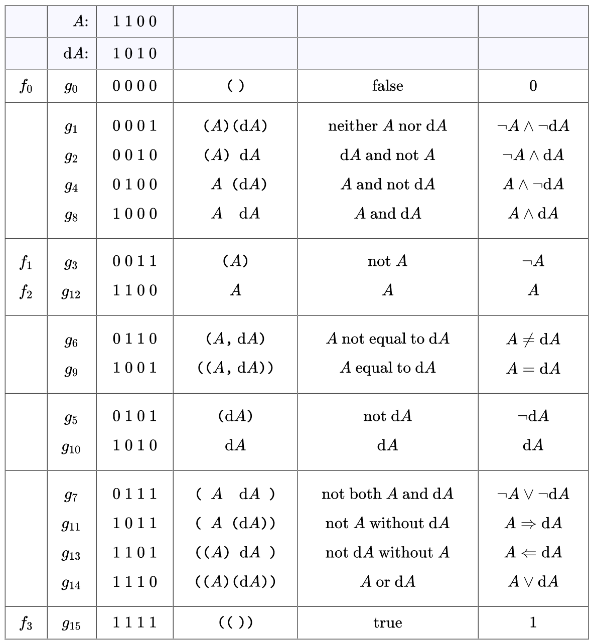
![[\mathrm{E}\mathcal{X}] = [A, \mathrm{d}A].](https://s0.wp.com/latex.php?latex=%5B%5Cmathrm%7BE%7D%5Cmathcal%7BX%7D%5D+%3D+%5BA%2C+%5Cmathrm%7Bd%7DA%5D.&bg=ffffff&fg=000000&s=0&c=20201002) Over the extended alphabet
Over the extended alphabet  of cardinality
  we generate the set of points
  of cardinality
  which bears the following chain of equivalent descriptions.
![\begin{array}{lll} \mathrm{E}X & = & \langle A, \mathrm{d}A \rangle \\[4pt] & = & \{ \texttt{(} A \texttt{)}, A \} ~\times~ \{ \texttt{(} \mathrm{d}A \texttt{)}, \mathrm{d}A \} \\[4pt] & = & \{ \texttt{(} A \texttt{)(} \mathrm{d}A \texttt{)},~ \texttt{(} A \texttt{)} \mathrm{d}A,~ A \texttt{(} \mathrm{d}A \texttt{)},~ A ~ \mathrm{d}A \}. \end{array}](https://s0.wp.com/latex.php?latex=%5Cbegin%7Barray%7D%7Blll%7D++%5Cmathrm%7BE%7DX+%26+%3D+%26+%5Clangle+A%2C+%5Cmathrm%7Bd%7DA+%5Crangle++%5C%5C%5B4pt%5D++%26+%3D+%26+%5C%7B+%5Ctexttt%7B%28%7D+A+%5Ctexttt%7B%29%7D%2C+A+%5C%7D+%7E%5Ctimes%7E+%5C%7B+%5Ctexttt%7B%28%7D+%5Cmathrm%7Bd%7DA+%5Ctexttt%7B%29%7D%2C+%5Cmathrm%7Bd%7DA+%5C%7D++%5C%5C%5B4pt%5D++%26+%3D+%26+%5C%7B+%5Ctexttt%7B%28%7D+A+%5Ctexttt%7B%29%28%7D+%5Cmathrm%7Bd%7DA+%5Ctexttt%7B%29%7D%2C%7E++%5Ctexttt%7B%28%7D+A+%5Ctexttt%7B%29%7D+%5Cmathrm%7Bd%7DA%2C%7E++A+%5Ctexttt%7B%28%7D+%5Cmathrm%7Bd%7DA+%5Ctexttt%7B%29%7D%2C%7E++A+%7E+%5Cmathrm%7Bd%7DA+%5C%7D.++%5Cend%7Barray%7D&bg=ffffff&fg=000000&s=0&c=20201002)
 at root isomorphic to
  An element of
 ![\mathrm{E}X^\bullet = [A, \mathrm{d}A]](https://s0.wp.com/latex.php?latex=%5Cmathrm%7BE%7DX%5E%5Cbullet+%3D+%5BA%2C+%5Cmathrm%7Bd%7DA%5D&bg=ffffff&fg=000000&s=0&c=20201002) the basic dispositions in
the basic dispositions in  each of type
  There are
  propositions in
  as detailed in the following Table.
 Thus the first set of propositions
  is automatically embedded in the present set
  and the corresponding inclusions are indicated at the far left margin of the Table.
 ruled out by the dynamic law
  then what remains is the quotient structure shown in the following Figure. The picture makes it easy to see how the dynamically allowable portion of the universe is partitioned between the respective holdings of
  and
and  As it happens, the fact might have been expressed “right off the bat” by an equivalent formulation of the differential law, one which uses the exclusive disjunction to state the law as
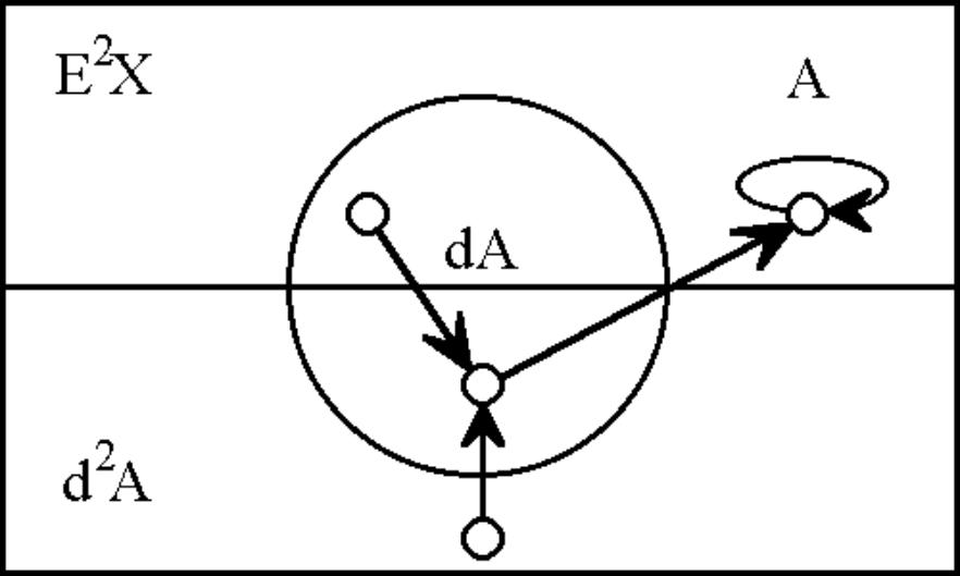

 is one‑dimensional we can easily fit the second order extension
  within the compass of a single venn diagram, charting the pair of converging trajectories as shown in the following Figure.
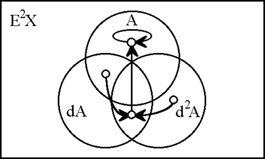

 suppose we are given the initial condition
  and the second order differential law
  Since the equation
  we may infer two possible trajectories, as shown in the following Table.

 is a stable attractor or terminal condition for both starting points.
 are changed or unchanged in the next moment. To know that one would have to determine
  and so on, pursuing an infinite regress. In order to rest with a finitely determinate system it is necessary to make an infinite assumption, for example, that
  for all
  greater than some fixed value
  Another way to escape the regress is through the provision of a dynamic law, in typical form making higher order differentials dependent on lower degrees and estates.
 If the feature
  may be taken as an attribute of the same object or state which tells it is changing significantly with respect to the property
  In practice, differential features acquire their meaning through a class of temporal inference rules.
 will be true in the next moment of observation. Taken all together we have the fourfold scheme of inference shown below.
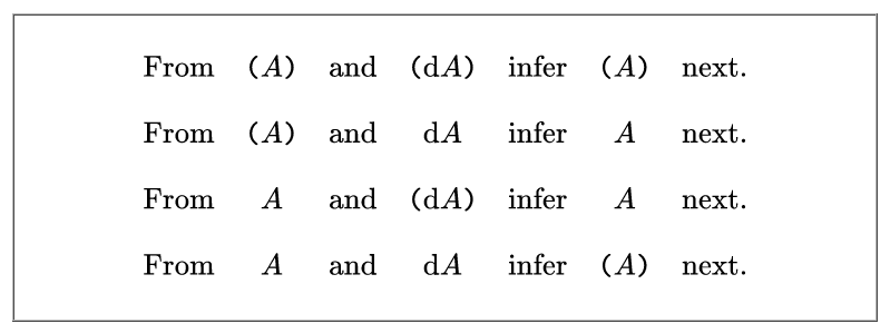
 be a logical basis containing one boolean variable or logical feature
  Corresponding to the basis
  which serves whenever we need to make explicit mention of the symbols used in our formulas and representations.
 of points (cells, vectors, interpretations) has cardinality
  and is isomorphic to
  Moreover,
  may be identified with the set of singular propositions
 is algebraically dual to
  Here,
Here,  is interpreted as denoting the constant function
  amounting to the linear proposition of rank
  while
while 
 of rank
  and
and  is understood as denoting the constant function
 propositions in the universe of discourse
 ![\mathcal{X}^\bullet = [\mathcal{X}],](https://s0.wp.com/latex.php?latex=%5Cmathcal%7BX%7D%5E%5Cbullet+%3D+%5B%5Cmathcal%7BX%7D%5D%2C&bg=ffffff&fg=000000&s=0&c=20201002) collectively forming the set
collectively forming the set 
