Differential Expansions of Propositions

Panoptic View • Difference Maps

In the previous section we computed what is variously described as the difference map, the difference proposition, or the local proposition of the proposition at the point where and

In the universe of discourse the four propositions indicating the “cells”, or the smallest distinguished regions of the universe, are called singular propositions.  These serve as an alternative notation for naming the points respectively.

Thus we can write so long as we know the frame of reference in force.

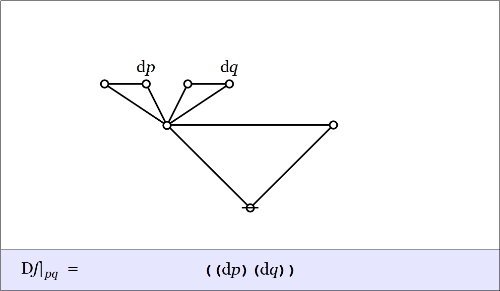
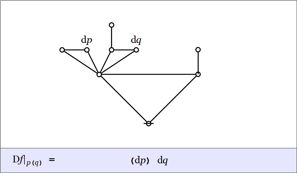
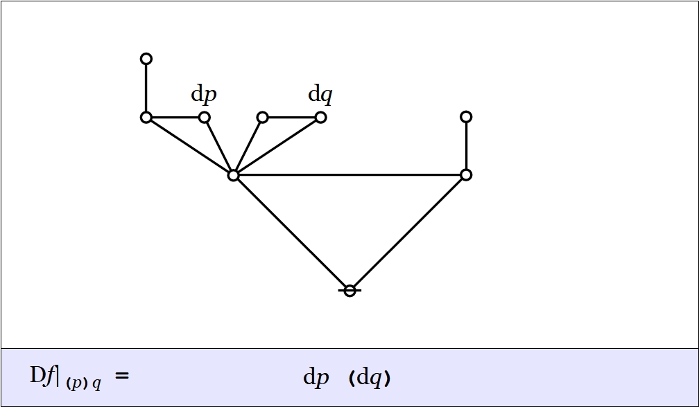
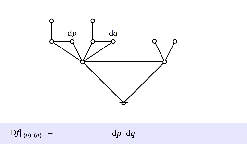
In the example the value of the difference proposition at each of the four points may be computed in graphical fashion as shown below.

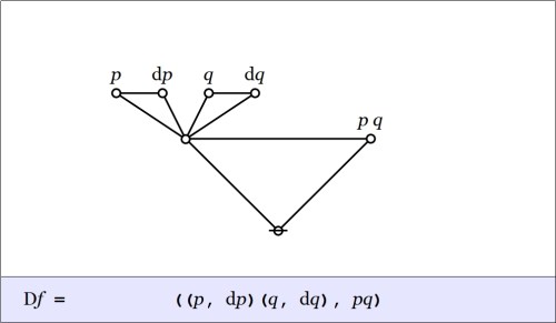
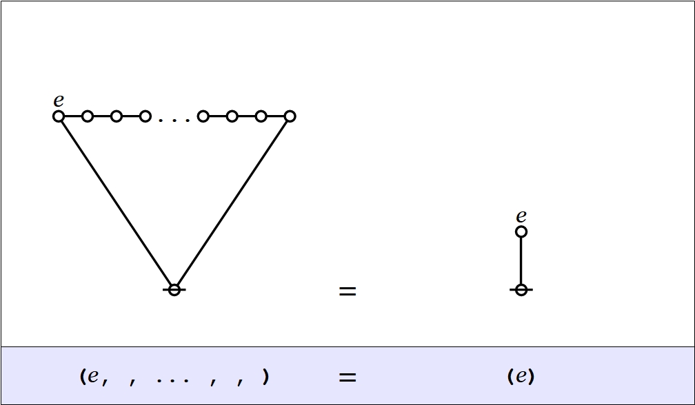
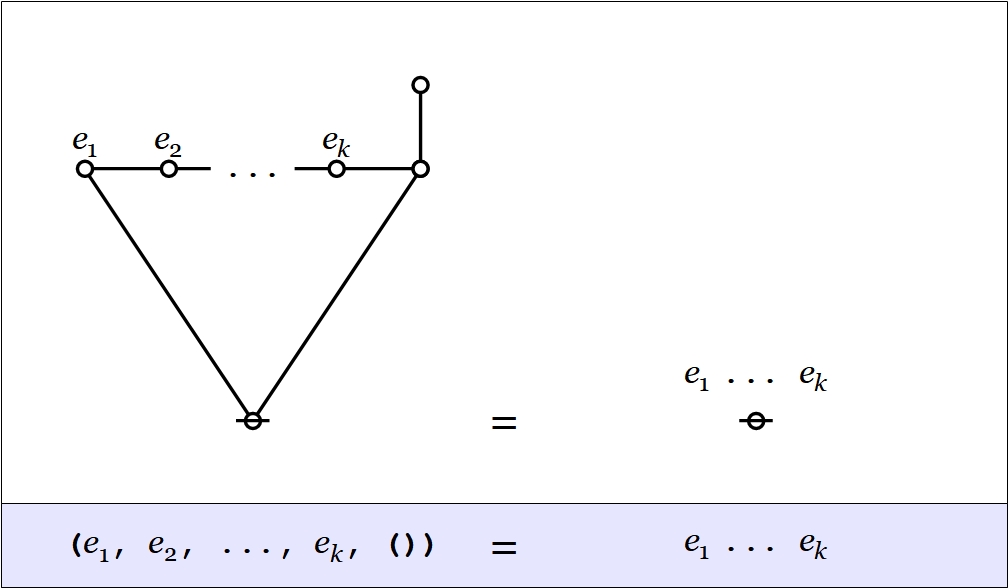
The easy way to visualize the values of these graphical expressions is just to notice the following equivalents.

Laying out the arrows on the augmented venn diagram, one gets a picture of a differential vector field.

The Figure shows the points of the extended universe indicated by the difference map namely, the following six points or singular propositions.

The information borne by should be clear enough from a survey of these six points — they tell you what you have to do from each point of in order to change the value borne by that is, the move you have to make in order to reach a point where the value of the proposition is different from what it is where you started.

We have been studying the action of the difference operator on propositions of the form as illustrated by the example which is known in logic as the conjunction of and   The resulting difference map is a (first order) differential proposition, that is, a proposition of the form

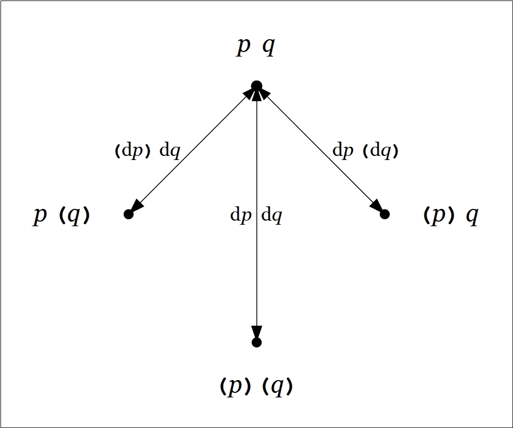
The augmented venn diagram shows how the models or satisfying interpretations of distribute over the extended universe of discourse   Abstracting from that picture, the difference map can be represented in the form of a digraph or directed graph, one whose points are labeled with the elements of and whose arrows are labeled with the elements of as shown in the following Figure.

Any proposition worth its salt can be analyzed from many different points of view, any one of which has the potential to reveal previously unsuspected aspects of the proposition’s meaning.  We will encounter more and more of these alternative readings as we go.

cc: Category Theory • Cybernetics • Ontolog • Structural Modeling • Systems Science
cc: FB | Differential Logic • Laws of Form • Peirce (1) (2) (3) (4)