Differential Expansions of Propositions

Worm’s Eye View

Let’s run through the initial example again, keeping an eye on the meanings of the formulas which develop along the way.  We begin with a proposition or a boolean function whose venn diagram and cactus graph are shown below.

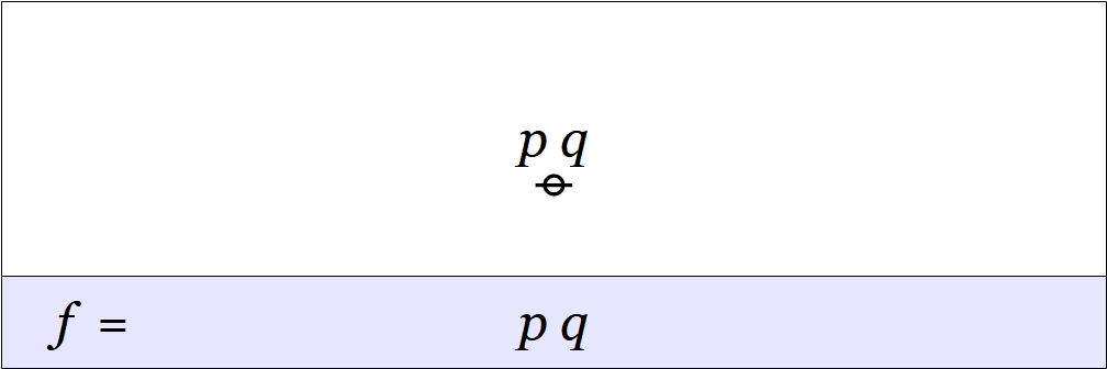
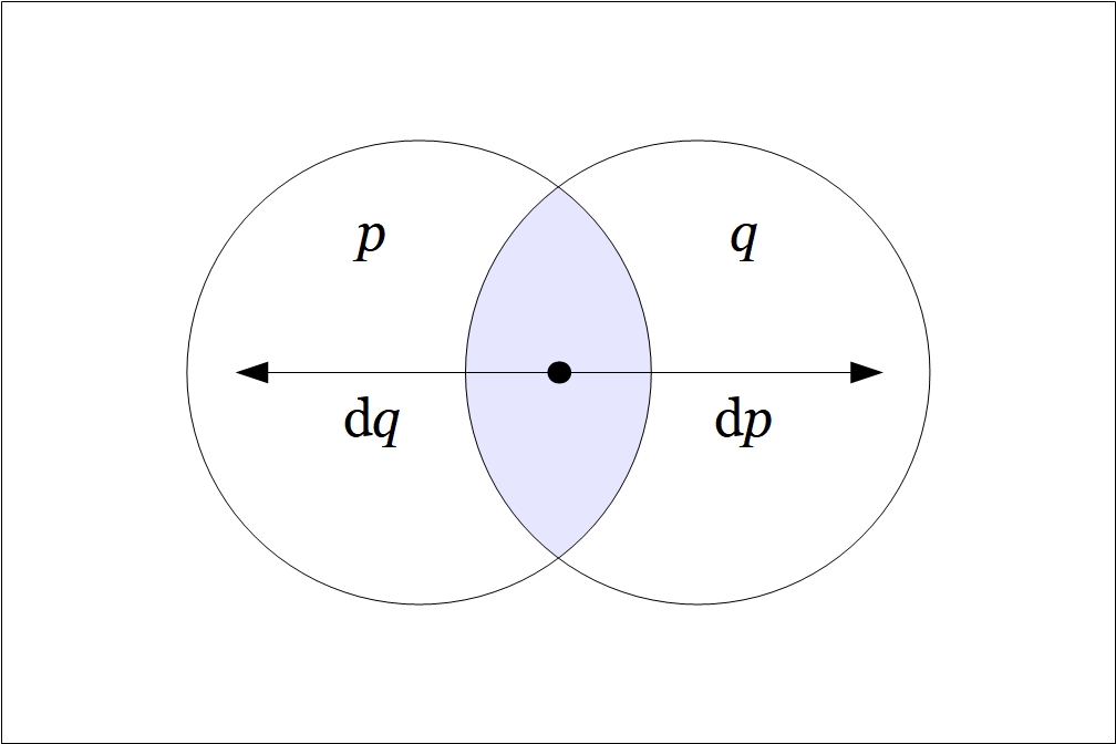
A function like this has an abstract type and a concrete type.  The abstract type is what we invoke when we write things like 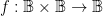or   The concrete type takes into account the qualitative dimensions or “units” of the case, which can be explained as follows.

Let be the set of values
Let be the set of values

Then interpret the usual propositions about as functions of the concrete type

We are going to consider various operators on these functions.  An operator is a function which takes one function into another function

The first couple of operators we need to consider are logical analogues of two which play a founding role in the classical finite difference calculus, namely:

The difference operator written here as
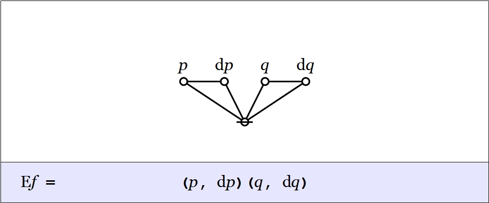
The enlargement operator, written here as

These days, is more often called the shift operator.

In order to describe the universe in which these operators operate, it is necessary to enlarge the original universe of discourse.  Starting from the initial space its (first order) differential extension is constructed according to the following specifications.

where:

The interpretations of these new symbols can be diverse, but the easiest option for now is just to say means “change ” and means “change ”.

Drawing a venn diagram for the differential extension requires four logical dimensions, but it is possible to project a suggestion of what the differential features and are about on the 2-dimensional base space by drawing arrows crossing the boundaries of the basic circles in the venn diagram for reading an arrow as if it crosses the boundary between and in either direction and reading an arrow as if it crosses the boundary between and in either direction, as indicated in the following figure.

Propositions are formed on differential variables, or any combination of ordinary logical variables and differential logical variables, in the same ways propositions are formed on ordinary logical variables alone.  For example, the proposition says the same thing as in other words, there is no change in without a change in

Given the proposition over the space the (first order) enlargement of is the proposition over the differential extension defined by the following formula.

In the example the enlargement is computed as follows.

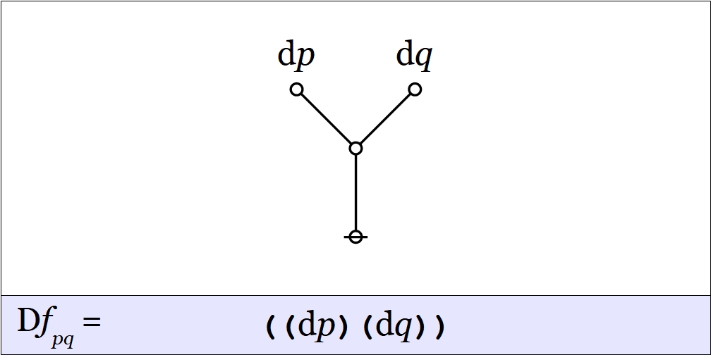
Given the proposition over the (first order) difference of is the proposition over defined by the formula or, written out in full:

In the example the difference is computed as follows.

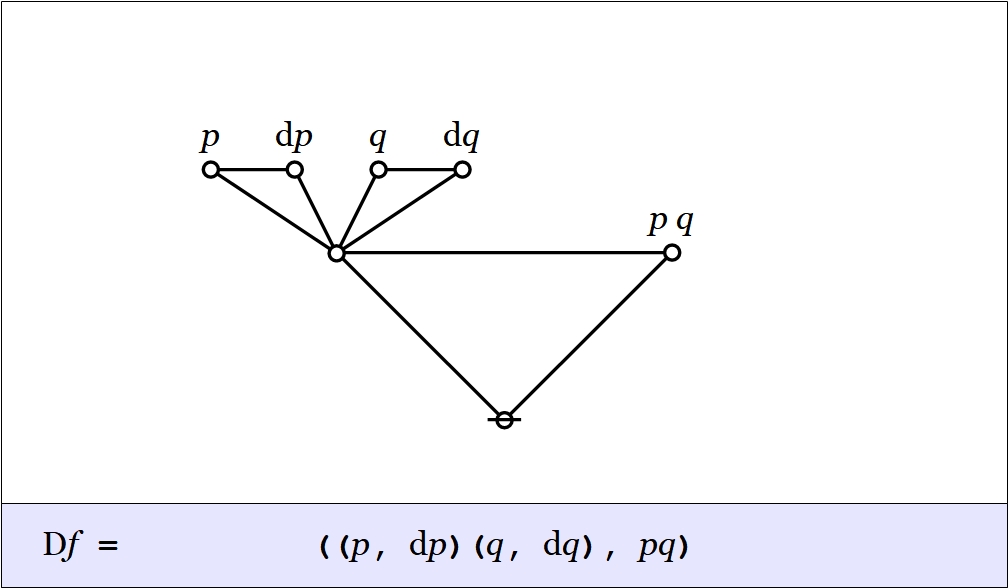
At the end of the previous section we evaluated this first order difference of conjunction at a single location in the universe of discourse, namely, at the point picked out by the singular proposition in terms of coordinates, at the place where and   This evaluation is written in the form or and we arrived at the locally applicable law which may be stated and illustrated as follows.

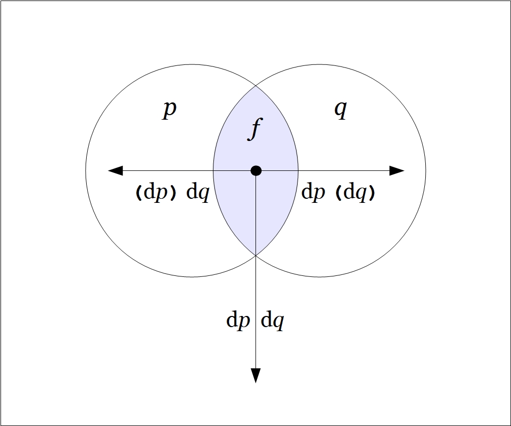
The venn diagram shows the analysis of the inclusive disjunction into the following exclusive disjunction.

The differential proposition may be read as saying “change or change or both”.  And this can be recognized as just what you need to do if you happen to find yourself in the center cell and require a complete and detailed description of ways to escape it.

cc: Category Theory • Cybernetics • Ontolog • Structural Modeling • Systems Science
cc: FB | Differential Logic • Laws of Form • Peirce (1) (2) (3) (4)