The enlargement or shift operator  exhibits a wealth of interesting and useful properties in its own right, so it pays to examine a few of the more salient features playing out on the surface of our initial example,
A suitably generic definition of the extended universe of discourse is afforded by the following set‑up.
![\begin{array}{cccl} \text{Let} & X & = & X_1 \times \ldots \times X_k. \\[6pt] \text{Let} & \mathrm{d}X & = & \mathrm{d}X_1 \times \ldots \times \mathrm{d}X_k. \\[6pt] \text{Then} & \mathrm{E}X & = & X \times \mathrm{d}X \\[6pt] & & = & X_1 \times \ldots \times X_k ~\times~ \mathrm{d}X_1 \times \ldots \times \mathrm{d}X_k \end{array}](https://s0.wp.com/latex.php?latex=%5Cbegin%7Barray%7D%7Bcccl%7D++%5Ctext%7BLet%7D+%26+X+%26+%3D+%26+X_1+%5Ctimes+%5Cldots+%5Ctimes+X_k.++%5C%5C%5B6pt%5D++%5Ctext%7BLet%7D+%26+%5Cmathrm%7Bd%7DX+%26+%3D+%26+%5Cmathrm%7Bd%7DX_1+%5Ctimes+%5Cldots+%5Ctimes+%5Cmathrm%7Bd%7DX_k.++%5C%5C%5B6pt%5D++%5Ctext%7BThen%7D+%26+%5Cmathrm%7BE%7DX+%26+%3D+%26+X+%5Ctimes+%5Cmathrm%7Bd%7DX++%5C%5C%5B6pt%5D++%26+%26+%3D+%26+X_1+%5Ctimes+%5Cldots+%5Ctimes+X_k+%7E%5Ctimes%7E+%5Cmathrm%7Bd%7DX_1+%5Ctimes+%5Cldots+%5Ctimes+%5Cmathrm%7Bd%7DX_k++%5Cend%7Barray%7D&bg=ffffff&fg=000000&s=0&c=20201002)
For a proposition of the form  the (first order) enlargement of
  is the proposition
  defined by the following equation.

The differential variables  are boolean variables of the same type as the ordinary variables
  Although it is conventional to distinguish the (first order) differential variables with the operational prefix
  this way of notating differential variables is entirely optional. It is their existence in particular relations to the initial variables, not their names, which defines them as differential variables.
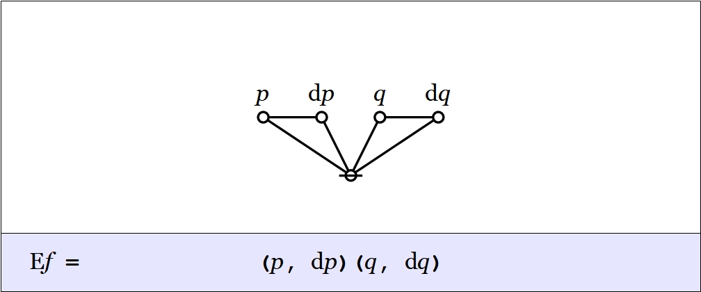
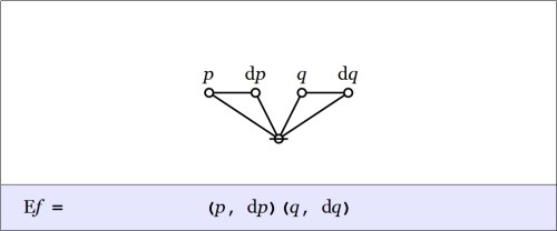
In the example of logical conjunction,  the enlargement
  is formulated as follows.

Given that this expression uses nothing more than the boolean ring operations of addition and multiplication, it is permissible to “multiply things out” in the usual manner to arrive at the following result.

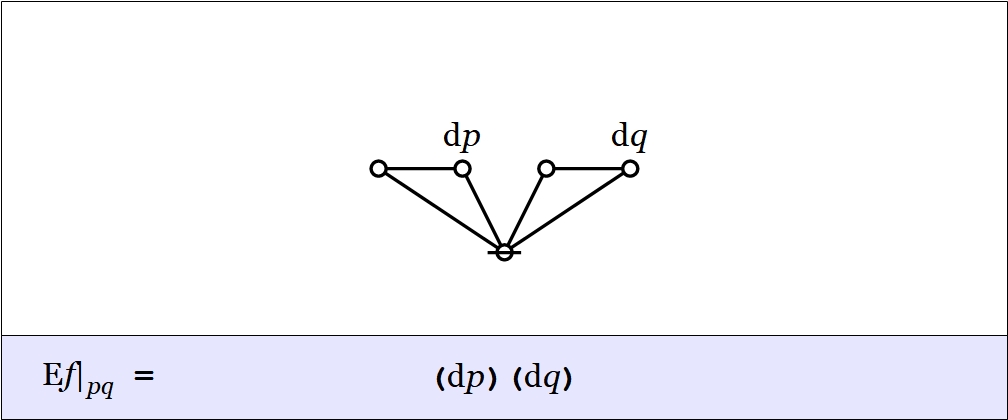
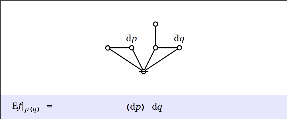
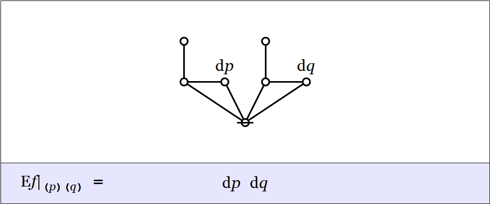
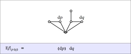
To understand what the enlarged or shifted proposition means in logical terms, it serves to go back and analyze the above expression for in the same way we did for  To that end, the value of
  at each
  may be computed in graphical fashion as shown below.


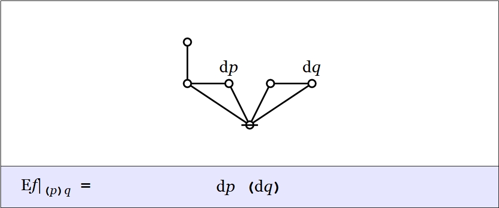
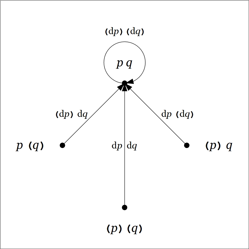
Collating the data of this analysis yields a boolean expansion or disjunctive normal form (DNF) equivalent to the enlarged proposition 

Here is a summary of the result, illustrated by means of a digraph picture, where the “no change” element  is drawn as a loop at the point
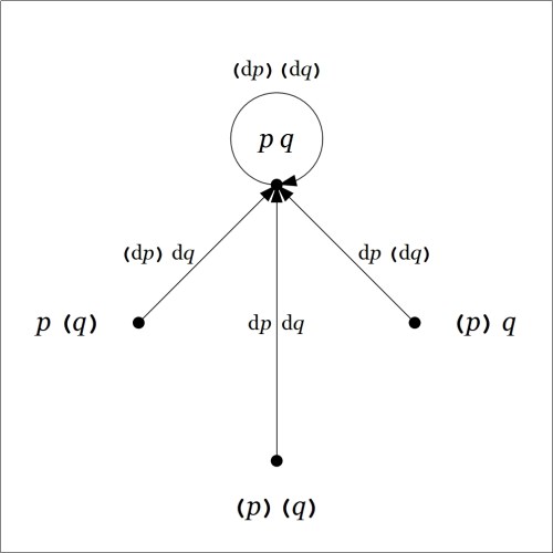
![\begin{array}{rcccccc} f & = & p & \cdot & q \\[4pt] \mathrm{E}f & = & p & \cdot & q & \cdot & \texttt{(} \mathrm{d}p \texttt{)(} \mathrm{d}q \texttt{)} \\[4pt] & + & p & \cdot & \texttt{(} q \texttt{)} & \cdot & \texttt{(} \mathrm{d}p \texttt{)} \texttt{~} \mathrm{d}q \texttt{~} \\[4pt] & + & \texttt{(} p \texttt{)} & \cdot & q & \cdot & \texttt{~} \mathrm{d}p \texttt{~} \texttt{(} \mathrm{d}q \texttt{)} \\[4pt] & + & \texttt{(} p \texttt{)} & \cdot & \texttt{(} q \texttt{)} & \cdot & \mathrm{d}p \texttt{~~} \mathrm{d}q \end{array}](https://s0.wp.com/latex.php?latex=%5Cbegin%7Barray%7D%7Brcccccc%7D++f+%26+%3D+%26+p++%26+%5Ccdot+%26+q++%5C%5C%5B4pt%5D++%5Cmathrm%7BE%7Df+%26+%3D+%26+p++%26+%5Ccdot+%26++q++%26+%5Ccdot+%26++%5Ctexttt%7B%28%7D+%5Cmathrm%7Bd%7Dp+%5Ctexttt%7B%29%28%7D+%5Cmathrm%7Bd%7Dq+%5Ctexttt%7B%29%7D++%5C%5C%5B4pt%5D++%26+%2B+%26++p++%26+%5Ccdot+%26+%5Ctexttt%7B%28%7D+q+%5Ctexttt%7B%29%7D++%26+%5Ccdot+%26++%5Ctexttt%7B%28%7D+%5Cmathrm%7Bd%7Dp+%5Ctexttt%7B%29%7D+%5Ctexttt%7B%7E%7D+%5Cmathrm%7Bd%7Dq+%5Ctexttt%7B%7E%7D++%5C%5C%5B4pt%5D++%26+%2B+%26++%5Ctexttt%7B%28%7D+p+%5Ctexttt%7B%29%7D+%26+%5Ccdot+%26++q++%26+%5Ccdot+%26++%5Ctexttt%7B%7E%7D+%5Cmathrm%7Bd%7Dp+%5Ctexttt%7B%7E%7D+%5Ctexttt%7B%28%7D+%5Cmathrm%7Bd%7Dq+%5Ctexttt%7B%29%7D++%5C%5C%5B4pt%5D++%26+%2B+%26++%5Ctexttt%7B%28%7D+p+%5Ctexttt%7B%29%7D+%26+%5Ccdot+%26+%5Ctexttt%7B%28%7D+q+%5Ctexttt%7B%29%7D++%26+%5Ccdot+%26+%5Cmathrm%7Bd%7Dp+%5Ctexttt%7B%7E%7E%7D+%5Cmathrm%7Bd%7Dq++%5Cend%7Barray%7D&bg=ffffff&fg=000000&s=0&c=20201002)
We may understand the enlarged proposition as telling us all the ways of reaching a model of the proposition from the points of the universe 
cc: Category Theory • Cybernetics • Ontolog • Structural Modeling • Systems Science
cc: FB | Differential Logic • Laws of Form • Peirce (1) (2) (3) (4)

 corresponding to the logical conjunction
  and examined how the differential operators
  act on
  Each differential operator takes a boolean function of two variables
  and gives back a boolean function of four variables,
  and
and 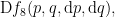 respectively.
 means
means  But usually people have something more pragmatic or rhetorical in mind than pure logic would require, something like enthymeme.
 with the causal order
  whereas it’s more like the reverse of that. In more complex settings we usually have the architectonic sense in mind, and that is what I sensed in the case of the normative sciences. Viewed with regard to their bases, logic is a special case of ethics and ethics is a special case of aesthetics, but with regard to their level of oversight, aesthetics must submit to ethical control and ethics must submit to logical control.
 means
means  See the following passage and commentary.
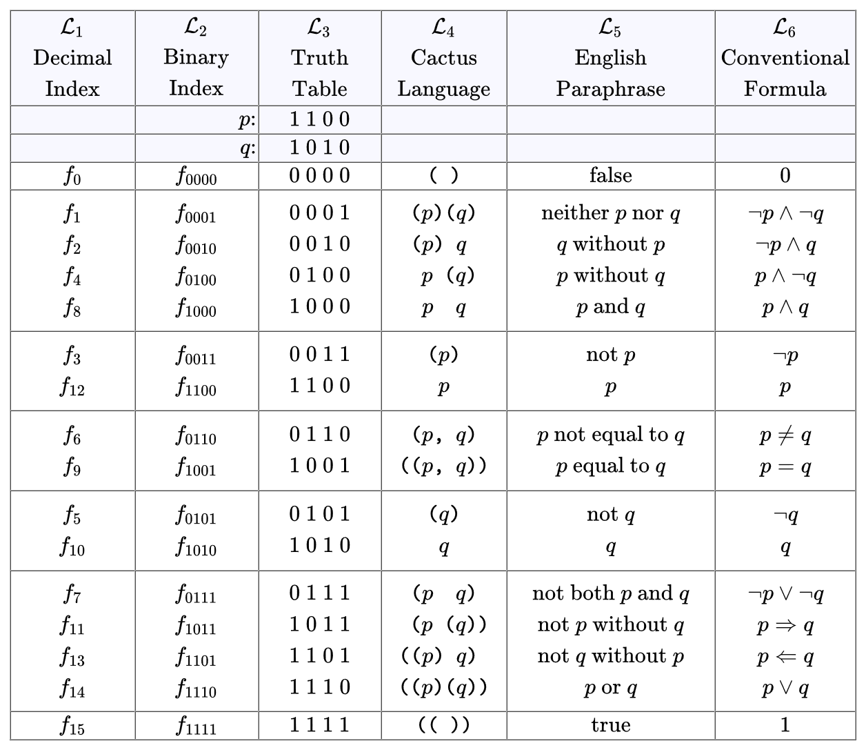
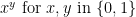 means the same thing as
  as one can tell by comparing the following two operation tables.
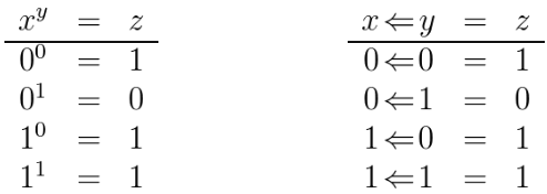
 and abstract type
  Our inquiry into the differential aspects of logical conjunction will pay dividends as we study the actions of