
Peirce’s 1870 “Logic of Relatives” • Comment 12.3
We now have two ways of computing a logical involution raising a dyadic relative term to the power of a monadic absolute term, for example, 
The first method applies set-theoretic operations to the extensions of absolute and relative terms, expressing the denotation of the term
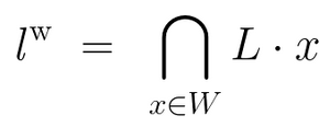
The second method operates in the matrix representation, expressing the value of the matrix 


Abstract formulas like these are more easily grasped with the aid of a concrete example and a picture of the relations involved.
Involution Example 1
Consider a universe of discourse 
![\begin{array}{*{15}{c}} X & = & \{ & a, & b, & c, & d, & e, & f, & g, & h, & i & \} \\[6pt] W & = & \{ & d, & f & \} \\[6pt] L & = & \{ & b\!:\!a, & b\!:\!c, & c\!:\!b, & c\!:\!d, & e\!:\!d, & e\!:\!e, & e\!:\!f, & g\!:\!f, & g\!:\!h, & h\!:\!g, & h\!:\!i & \} \end{array}](https://s0.wp.com/latex.php?latex=%5Cbegin%7Barray%7D%7B%2A%7B15%7D%7Bc%7D%7D++X+%26+%3D+%26+%5C%7B+%26+a%2C+%26+b%2C+%26+c%2C+%26+d%2C+%26+e%2C+%26+f%2C+%26+g%2C+%26+h%2C+%26+i+%26+%5C%7D++%5C%5C%5B6pt%5D++W+%26+%3D+%26+%5C%7B+%26+d%2C+%26+f+%26+%5C%7D++%5C%5C%5B6pt%5D++L+%26+%3D+%26+%5C%7B+%26+b%5C%21%3A%5C%21a%2C+%26+b%5C%21%3A%5C%21c%2C+%26+c%5C%21%3A%5C%21b%2C+%26+c%5C%21%3A%5C%21d%2C+%26+e%5C%21%3A%5C%21d%2C+%26+e%5C%21%3A%5C%21e%2C+%26+e%5C%21%3A%5C%21f%2C+%26+g%5C%21%3A%5C%21f%2C+%26+g%5C%21%3A%5C%21h%2C+%26+h%5C%21%3A%5C%21g%2C+%26+h%5C%21%3A%5C%21i+%26+%5C%7D++%5Cend%7Barray%7D&bg=ffffff&fg=000000&s=1&c=20201002)
Figure 55 shows the placement of 


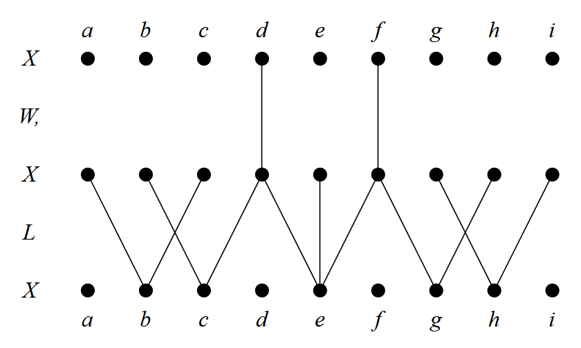

To highlight the role of 

Computing the denotation of

With the above Figure in mind, we can visualize the computation of 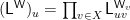
- Pick a specific
- Pan across the elements
in the middle row of the Figure.
- If
otherwise
- If
otherwise
- Compute the value
for each
- If any of the values
is
then the product
is
otherwise it is


As a general observation, we know the value of 


Running through the program for each 


Resources
- Peirce’s 1870 Logic of Relatives • Part 1 • Part 2 • Part 3 • References
- Logic Syllabus • Relational Concepts • Relation Theory • Relative Term
cc: Cybernetics • Ontolog Forum • Structural Modeling • Systems Science
cc: FB | Peirce Matters • Laws of Form • Peirce List (1) (2) (3) (4) (5) (6) (7)

Pingback: Survey of Relation Theory • 3 | Inquiry Into Inquiry
Pingback: Peirce’s 1870 “Logic Of Relatives” • Overview | Inquiry Into Inquiry
Pingback: Peirce’s 1870 “Logic Of Relatives” • Comment 1 | Inquiry Into Inquiry
Pingback: Survey of Relation Theory • 4 | Inquiry Into Inquiry
Pingback: Survey of Relation Theory • 5 | Inquiry Into Inquiry
Pingback: Survey of Relation Theory • 6 | Inquiry Into Inquiry
Pingback: Survey of Relation Theory • 7 | Inquiry Into Inquiry
Pingback: Survey of Relation Theory • 8 | Inquiry Into Inquiry
Pingback: Peirce’s 1885 “Algebra of Logic” • Discussion 1 | Inquiry Into Inquiry
Pingback: Peirce’s 1885 “Algebra of Logic” • Discussion 2 | Inquiry Into Inquiry
Pingback: Survey of Relation Theory • 9 | Inquiry Into Inquiry