Inquiry Into Inquiry

Differential Propositional Calculus • Discussion 1

Posted on March 12, 2020 by Jon Awbrey

The most fundamental concept in cybernetics is that of “difference”, either that two things are recognisably different or that one thing has changed with time.

W. Ross Ashby • An Introduction to Cybernetics

Re: Cybernetics Communications • Klaus Krippendorff

KK:: To me, differences are the result of drawing distinctions. They don’t exist unless you actively draw them. So, the act of drawing distinctions is more fundamental than the differences thereby created.

I often return to that line from Ashby. This time I thought it made an apt segue from the scene of propositional calculus, where universes of discourse are ruled by collections of distinctive features, to the differential extension of propositional calculus, which enables us to describe trajectories within and transformations between our logical universes.

So I agree with Klaus Krippendorff about “which came first”, the distinctions drawn or the states distinguished in space or time. The primitive character of distinctions is especially salient in this setting since our formalism for propositional calculus is built on the forms of distinction pioneered by C.S. Peirce and augmented by George Spencer Brown.

Resources

Differential Propositional Calculus • Part 1 • Part 2
Differential Logic • Part 1 • Part 2 • Part 3
Differential Logic and Dynamic Systems
• Part 1 • Part 2 • Part 3 • Part 4 • Part 5

cc: Cybernetics • Ontolog • Peirce List (1) (2) • Structural Modeling • Systems Science

Posted in Amphecks, Boolean Functions, C.S. Peirce, Cactus Graphs, Category Theory, Change, Computational Complexity, Cybernetics, Differential Analytic Turing Automata, Differential Calculus, Differential Logic, Discrete Dynamics, Dynamical Systems, Equational Inference, Functional Logic, Gradient Descent, Graph Theory, Group Theory, Hologrammautomaton, Indicator Functions, Logic, Logical Graphs, Mathematical Models, Mathematics, Minimal Negation Operators, Painted Cacti, Peirce, Propositional Calculus, Propositional Equation Reasoning Systems, Time, Visualization | Tagged Amphecks, Boolean Functions, C.S. Peirce, Cactus Graphs, Category Theory, Change, Computational Complexity, Cybernetics, Differential Analytic Turing Automata, Differential Calculus, Differential Logic, Discrete Dynamics, Dynamical Systems, Equational Inference, Functional Logic, Gradient Descent, Graph Theory, Group Theory, Hologrammautomaton, Indicator Functions, Logic, Logical Graphs, Mathematical Models, Mathematics, Minimal Negation Operators, Painted Cacti, Peirce, Propositional Calculus, Propositional Equation Reasoning Systems, Time, Visualization | 13 Comments

Abduction, Deduction, Induction, Analogy, Inquiry • 28

Posted on March 10, 2020 by Jon Awbrey

Re: Ontolog Forum • Michael DeBellis • Adrian Walker

MDB:: I’m currently auditing a fascinating seminar at Berkeley on Semiotics and Information Theory. Mostly we are focusing on C.S. Peirce although we’ve also explored other theories such as Shannon’s Information Theory. As we were discussing abduction, the history of the idea, how it compares with induction and deduction, etc. someone asked me about the uses of Abduction in AI and computer science.

Just off hand, here’s a batch of blog and wiki links relating to “Abductive Intelligence”.

Survey of Abduction, Deduction, Induction, Analogy, Inquiry

My first encounters with abductive reasoning in computational contexts go back to mentions of Peirce by Warren S. McCulloch and early implementations by Pople, et al. Here’s a few notes on those.

Warren S. McCulloch • What Is a Number, that a Man May Know It, and a Man, that He May Know a Number?
Abduction, Deduction, Induction, Analogy, Inquiry • (15) • (23)

All through 1995 I worked on a graduate project in systems engineering at Oakland University developing my ideas about Inquiry Driven Systems. A project report I wrote on Peirce’s treatments of analogy and inquiry includes a discussion of the logical inferences involved in the abductive and deductive steps. There’s a copy of that at the following location: Functional Logic • Inquiry and Analogy

AW:: Interestingly, this topic [abductive inference] overlaps with planning.

Exactly. Resolving a surprise through an explanation and solving a problem through a plan of action are dual species of inquiry in general.

This is one of the themes at the top of my work on Inquiry Driven Systems. See, for example, the statement of research interests I submitted with my application to grad school back in the early 90s.

Prospects for Inquiry Driven Systems

Topos : Rudiments and Immediate Resources

This inquiry is guided by two questions that express themselves in many different guises. In their most laconic and provocative style, self-referent but not purely so, they typically bring a person to ask:

Why am I asking this question?
How will I answer this question?

Cast in with a pool of other questions these two often act as efficient catalysts of the inquiry process, precipitating and organizing what results. Expanded into general terms these queries become tantamount to asking:

What accumulated funds and immediate series of experiences lead up to the moment of surprise that causes the asking of a question?
What operational resources and planned sequences of actions lead on to the moment of solution that allows the ending of a problem?

Phrased in systematic terms, they ask yet again:

What capacity enables a system to exist in states of question?
What competence enables a system to exit from its problem states?

cc: Cybernetics • Ontolog Forum • Peirce List • Structural Modeling • Systems Science

Posted in Abduction, Analogy, Aristotle, Artificial Intelligence, C.S. Peirce, Deduction, Induction, Inquiry, Inquiry Driven Systems, Intelligent Systems Engineering, Logic, Mental Models, Peirce, Scientific Method, Semiotics, Systems | Tagged Abduction, Analogy, Aristotle, Artificial Intelligence, C.S. Peirce, Deduction, Induction, Inquiry, Inquiry Driven Systems, Intelligent Systems Engineering, Logic, Mental Models, Peirce, Scientific Method, Semiotics, Systems | 5 Comments

Pragmatic Truth • Discussion 22

Posted on March 9, 2020 by Jon Awbrey

Re: Systems Science • Scott Jackson

Discussions of “thinking and flawed decisions” arising in the Systems Science Working Group naturally brought the topic of Pragmatic Truth and all its bedeviled vicissitudes back to this Peircean’s mind.

I have often observed how belief systems act in a way like immune systems, generating “antibodies” to combat the “antigens” of any ideas beyond their comfort zones.

Elsewhere, I described these phenomena under the heading of Information Resistance.

The hardest thing to understand about information is people’s resistance to it.

The locus pragmaticus for the study of belief systems and the impact of information and inquiry on them is C.S. Peirce’s “The Fixation of Belief”. See the preceding post in this series for comment and links.

Reference

Peirce, C.S. (1877), “The Fixation of Belief”, Popular Science Monthly 12, 1–15.

Resources

cc: Cybernetics • Ontolog • Peirce List (1) (2) • Structural Modeling • Systems Science

Posted in Aristotle, C.S. Peirce, Coherence, Concordance, Congruence, Consensus, Convergence, Correspondence, Dewey, Fixation of Belief, Information, Inquiry, John Dewey, Kant, Logic, Logic of Science, Method, Peirce, Philosophy, Pragmatic Maxim, Pragmatism, Semiotics, Sign Relations, Triadic Relations, Truth, Truth Theory, William James | Tagged Aristotle, C.S. Peirce, Coherence, Concordance, Congruence, Consensus, Convergence, Correspondence, Dewey, Fixation of Belief, Information, Inquiry, John Dewey, Kant, Logic, Logic of Science, Method, Peirce, Philosophy, Pragmatic Maxim, Pragmatism, Semiotics, Sign Relations, Triadic Relations, Truth, Truth Theory, William James | 5 Comments

Differential Propositional Calculus • 8

Posted on March 7, 2020 by Jon Awbrey

Differential Extensions

An initial universe of discourse $A^\bullet$ supplies the groundwork for any number of further extensions, beginning with the first order differential extension $\mathrm{E}A^\bullet.$ The construction of $\mathrm{E}A^\bullet$ can be described in the following stages.

The initial alphabet $\mathfrak{A} = \{ ``a_1", \ldots, ``a_n" \}$ is extended by a first order differential alphabet $\mathrm{d}\mathfrak{A} = \{ ``\mathrm{d}a_1", \ldots, ``\mathrm{d}a_n" \}$ resulting in a first order extended alphabet $\mathrm{E}\mathfrak{A}$ defined as follows.

$\mathrm{E}\mathfrak{A} ~=~ \mathfrak{A} ~\cup~ \mathrm{d}\mathfrak{A} ~=~ \{ ``a_1", \ldots, ``a_n", ``\mathrm{d}a_1", \ldots, ``\mathrm{d}a_n" \}.$
The initial basis $\mathcal{A} = \{ a_1, \ldots, a_n \}$ is extended by a first order differential basis $\mathrm{d}\mathcal{A} = \{ \mathrm{d}a_1, \ldots, \mathrm{d}a_n \}$ resulting in a first order extended basis $\mathrm{E}\mathcal{A}$ defined as follows.

$\mathrm{E}\mathcal{A} ~=~ \mathcal{A} ~\cup~ \mathrm{d}\mathcal{A} ~=~ \{ a_1, \ldots, a_n, \mathrm{d}a_1, \ldots, \mathrm{d}a_n \}.$
The initial space $A = \langle a_1, \ldots, a_n \rangle$ is extended by a first order differential space or tangent space $\mathrm{d}A = \langle \mathrm{d}a_1, \ldots, \mathrm{d}a_n \rangle$ at each point of $A,$ resulting in a first order extended space or tangent bundle space $\mathrm{E}A$ defined as follows.

$\mathrm{E}A ~=~ A ~\times~ \mathrm{d}A ~=~ \langle \mathrm{E}\mathcal{A} \rangle ~=~ \langle \mathcal{A} \cup \mathrm{d}\mathcal{A} \rangle ~=~ \langle a_1, \ldots, a_n, \mathrm{d}a_1, \ldots, \mathrm{d}a_n \rangle.$
Finally, the initial universe $A^\bullet = [ a_1, \ldots, a_n ]$ is extended by a first order differential universe or tangent universe $\mathrm{d}A^\bullet = [ \mathrm{d}a_1, \ldots, \mathrm{d}a_n ]$ at each point of $A^\bullet,$ resulting in a first order extended universe or tangent bundle universe $\mathrm{E}A^\bullet$ defined as follows.

$\mathrm{E}A^\bullet ~=~ [ \mathrm{E}\mathcal{A} ] ~=~ [ \mathcal{A} ~\cup~ \mathrm{d}\mathcal{A} ] ~=~ [ a_1, \ldots, a_n, \mathrm{d}a_1, \ldots, \mathrm{d}a_n ].$

This gives $\mathrm{E}A^\bullet$ a type defined as follows.

$[ \mathbb{B}^n \times \mathbb{D}^n ] ~=~ (\mathbb{B}^n \times \mathbb{D}^n\ +\!\!\to \mathbb{B}) ~=~ (\mathbb{B}^n \times \mathbb{D}^n, \mathbb{B}^n \times \mathbb{D}^n \to \mathbb{B}).$

A proposition in a differential extension of a universe of discourse is called a differential proposition and forms the analogue of a system of differential equations in ordinary calculus. With these constructions, the first order extended universe $\mathrm{E}A^\bullet$ and the first order differential propositions $f : \mathrm{E}A \to \mathbb{B},$ we arrive at the foothills of differential logic.

Table 11 summarizes the notations needed to describe the first order differential extensions of propositional calculi in a systematic manner.

$\text{Table 11. Differential Extension} \stackrel{_\bullet}{} \text{Basic Notation}$

Resources

Logic Syllabus
Differential Propositional Calculus • Part 1 • Part 2

cc: Cybernetics • Ontolog Forum • Peirce List • Structural Modeling • Systems Science

Habitations

Posted on March 6, 2020 by Jon Awbrey

Our reach exceeds our rut and yet
We grasp but what we drag into it.

Re: Scott Aaronson • A Coronavirus Poem

Posted in Anthem, Anthematics, Mantra, Maxim, Meditation, Poetry, Reflection, Reverie, Sisyphus, Verse | Tagged Anthem, Anthematics, Mantra, Maxim, Meditation, Poetry, Reflection, Reverie, Sisyphus, Verse | Leave a comment

Differential Propositional Calculus • 7

Posted on March 5, 2020 by Jon Awbrey

Special Classes of Propositions (concl.)

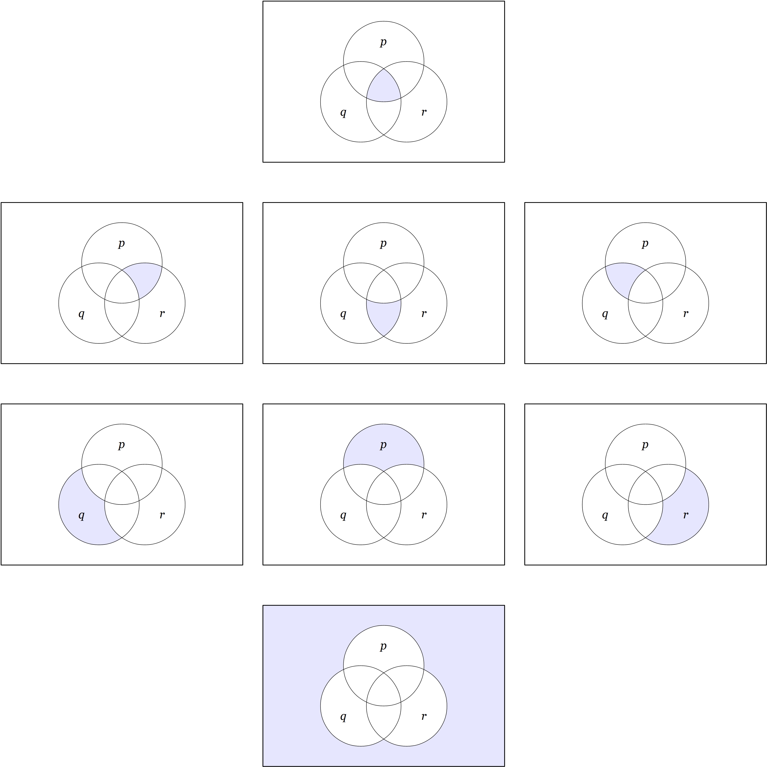
Last and literally least in extent, we examine the family of singular propositions in a 3-dimensional universe of discourse.

In our model of propositions as mappings of a universe of discourse to a set of two values, in other words, indicator functions of the form $f : X \to \mathbb{B},$ singular propositions are those singling out the minimal distinct regions of the universe, represented by single cells of the corresponding venn diagram.

Singular Propositions

In a universe of discourse based on three boolean variables, $p, q, r,$ there are $2^3 = 8$ singular propositions. Their venn diagrams are shown in Figure 10.

$\text{Figure 10.} ~~ \text{Singular Propositions} : \mathbb{B}^3 \to \mathbb{B}$

At the top is the venn diagram for the singular proposition of rank 3, corresponding to the boolean product $pqr$ and identical with the positive proposition of rank 3.

Next are the venn diagrams for the three singular propositions of rank 2, which may be expressed by the following three forms, respectively:

$pr \texttt{(} q \texttt{)}, \qquad qr \texttt{(} p \texttt{)}, \qquad pq \texttt{(} r \texttt{)}.$

Next are the three singular propositions of rank 1, which may be expressed by the following three forms, respectively:

$q \texttt{(} p \texttt{)(} r \texttt{)}, \qquad p \texttt{(} q \texttt{)(} r \texttt{)}, \qquad r \texttt{(} p \texttt{)(} q \texttt{)}.$

At the bottom is the singular proposition of rank 0, which may be expressed by the following form:

$\texttt{(} p \texttt{)(} q \texttt{)(} r \texttt{)}.$

Resources

Logic Syllabus
Differential Propositional Calculus • Part 1 • Part 2

cc: Cybernetics • Ontolog Forum • Peirce List • Structural Modeling • Systems Science

Differential Propositional Calculus • 6

Posted on March 2, 2020 by Jon Awbrey

Special Classes of Propositions (cont.)

Next we take up the family of positive propositions and follow the same plan as before, tracing the rule of their formation in the case of a 3-dimensional universe of discourse.

Positive Propositions

In a universe of discourse based on three boolean variables, $p, q, r,$ there are $2^3 = 8$ positive propositions, taking the shapes shown in Figure 9.

$\text{Figure 9.} ~~ \text{Positive Propositions} : \mathbb{B}^3 \to \mathbb{B}$

At the top is the venn diagram for the positive proposition of rank 3, corresponding to the boolean product or logical conjunction $pqr.$

Next are the venn diagrams for the three positive propositions of rank 2, corresponding to the three boolean products, $pr, qr, pq,$ respectively.

Next are the three positive propositions of rank 1, which are none other than the three basic propositions, $p, q, r.$

At the bottom is the positive proposition of rank 0, the everywhere true proposition or the constant $1$ function, which may be expressed by the form $\texttt{((}~\texttt{))}$ or by a simple $1.$

Resources

Logic Syllabus
Differential Propositional Calculus • Part 1 • Part 2

cc: Cybernetics • Ontolog Forum • Peirce List • Structural Modeling • Systems Science

Differential Propositional Calculus • 5

Posted on February 29, 2020 by Jon Awbrey

Special Classes of Propositions (cont.)

Let’s pause at this point and get a better sense of how our special classes of propositions are structured and how they relate to propositions in general. We can do this by recruiting our visual imaginations and drawing up a sufficient budget of venn diagrams for each family of propositions. The case for 3 variables is exemplary enough for a start.

Linear Propositions

One thing to keep in mind about these sums is that the values in $\mathbb{B} = \{ 0, 1 \}$ are added “modulo 2”, that is, in such a way that $1 + 1 = 0.$

In a universe of discourse based on three boolean variables, $p, q, r,$ the linear propositions take the shapes shown in Figure 8.

$\text{Figure 8.} ~~ \text{Linear Propositions} : \mathbb{B}^3 \to \mathbb{B}$

At the top is the venn diagram for the linear proposition of rank 3, which may be expressed by any one of the following three forms:

$\texttt{(} p \texttt{,(} q \texttt{,} r \texttt{))}, \qquad \texttt{((} p \texttt{,} q \texttt{),} r \texttt{)}, \qquad p + q + r.$

Next are the venn diagrams for the three linear propositions of rank 2, which may be expressed by the following three forms, respectively:

$\texttt{(} p \texttt{,} r \texttt{)}, \qquad \texttt{(} q \texttt{,} r \texttt{)}, \qquad \texttt{(} p \texttt{,} q \texttt{)}.$

Next are the three linear propositions of rank 1, which are none other than the three basic propositions, $p, q, r.$

At the bottom is the linear proposition of rank 0, the everywhere false proposition or the constant $0$ function, which may be expressed by the form $\texttt{(} ~ \texttt{)}$ or by a simple $0.$

Resources

Logic Syllabus
Differential Propositional Calculus • Part 1 • Part 2

cc: Cybernetics • Ontolog Forum • Peirce List • Structural Modeling • Systems Science

Differential Propositional Calculus • 4

Posted on February 25, 2020 by Jon Awbrey

Special Classes of Propositions

Before moving on, let’s unpack some of the assumptions, conventions, and implications involved in the array of concepts and notations introduced above.

A universe of discourse $A^\bullet = [a_1, \ldots, a_n]$ qualified by the logical features $a_1, \ldots, a_n$ is a set $A$ plus the set of all functions from the space $A$ to the boolean domain $\mathbb{B} = \{ 0, 1 \}.$ There are $2^n$ elements in $A,$ often pictured as the cells of a venn diagram or the nodes of a hypercube. There are $2^{2^n}$ possible functions from $A$ to $\mathbb{B},$ accordingly pictured as all the ways of painting the cells of a venn diagram or the nodes of a hypercube with a palette of two colors.

A logical proposition about the elements of $A$ is either true or false of each element in $A,$ while a function $f : A \to \mathbb{B}$ evaluates to $1$ or $0$ on each element of $A.$ The analogy between logical propositions and boolean-valued functions is close enough to adopt the latter as models of the former and simply refer to the functions $f : A \to \mathbb{B}$ as propositions about the elements of $A.$

The full set of propositions $f : A \to \mathbb{B}$ contains a number of smaller classes deserving of special attention.

A basic proposition in the universe of discourse $[a_1, \ldots, a_n]$ is one of the propositions in the set $\{ a_1, \ldots, a_n \}.$ There are of course exactly $n$ of these. Depending on the context, basic propositions may also be called coordinate propositions or simple propositions.

Among the $2^{2^n}$ propositions in $[a_1, \ldots, a_n]$ are several families numbering $2^n$ propositions each which take on special forms with respect to the basis $\{ a_1, \ldots, a_n \}.$ Three of these families are especially prominent in the present context, the linear, the positive, and the singular propositions. Each family is naturally parameterized by the coordinate $n$ -tuples in $\mathbb{B}^n$ and falls into $n + 1$ ranks, with a binomial coefficient $\tbinom{n}{k}$ giving the number of propositions having rank or weight $k$ in their class.

The linear propositions, $\{ \ell : \mathbb{B}^n \to \mathbb{B} \} = (\mathbb{B}^n \xrightarrow{\ell} \mathbb{B}),$ may be written as sums:

$\sum_{i=1}^n e_i ~=~ e_1 + \ldots + e_n ~\text{where}~ \left\{\begin{matrix} e_i = a_i \\ \text{or} \\ e_i = 0 \end{matrix}\right\} ~\text{for}~ i = 1 ~\text{to}~ n.$

The positive propositions, $\{ p : \mathbb{B}^n \to \mathbb{B} \} = (\mathbb{B}^n \xrightarrow{p} \mathbb{B}),$ may be written as products:

$\prod_{i=1}^n e_i ~=~ e_1 \cdot \ldots \cdot e_n ~\text{where}~ \left\{\begin{matrix} e_i = a_i \\ \text{or} \\ e_i = 1 \end{matrix}\right\} ~\text{for}~ i = 1 ~\text{to}~ n.$

The singular propositions, $\{ \mathbf{x} : \mathbb{B}^n \to \mathbb{B} \} = (\mathbb{B}^n \xrightarrow{s} \mathbb{B}),$ may be written as products:

$\prod_{i=1}^n e_i ~=~ e_1 \cdot \ldots \cdot e_n ~\text{where}~ \left\{\begin{matrix} e_i = a_i \\ \text{or} \\ e_i = \texttt{(} a_i \texttt{)} \end{matrix}\right\} ~\text{for}~ i = 1 ~\text{to}~ n.$

In each case the rank $k$ ranges from $0$ to $n$ and counts the number of positive appearances of the coordinate propositions $a_1, \ldots, a_n$ in the resulting expression. For example, when $n = 3$ the linear proposition of rank $0$ is $0,$ the positive proposition of rank $0$ is $1,$ and the singular proposition of rank $0$ is $\texttt{(} a_1 \texttt{)} \texttt{(} a_2 \texttt{)} \texttt{(} a_3 \texttt{)}.$

The basic propositions $a_i : \mathbb{B}^n \to \mathbb{B}$ are both linear and positive. So these two kinds of propositions, the linear and the positive, may be viewed as two different ways of generalizing the class of basic propositions.

Finally, it is important to note that all of the above distinctions are relative to the choice of a particular logical basis $\mathcal{A} = \{ a_1, \ldots, a_n \}.$ A singular proposition with respect to the basis $\mathcal{A}$ will not remain singular if $\mathcal{A}$ is extended by a number of new and independent features. Even if one keeps to the original set of pairwise options $\{ a_i \} \cup \{ \texttt{(} a_i \texttt{)} \}$ to pick out a new basis, the sets of linear propositions and positive propositions are both determined by the choice of basic propositions, and this whole determination is tantamount to the purely conventional choice of a cell as origin.

Resources

Logic Syllabus
Differential Propositional Calculus • Part 1 • Part 2

cc: Cybernetics • Ontolog Forum • Peirce List • Structural Modeling • Systems Science

Differential Propositional Calculus • 3

Posted on February 24, 2020 by Jon Awbrey

Formal Development

The preceding discussion outlined the ideas leading to the differential extension of propositional logic. The next task is to lay out the concepts and terminology needed to describe various orders of differential propositional calculi.

Elementary Notions

Logical description of a universe of discourse begins with a collection of logical signs. For simplicity in a first approach we assume the signs are collected in the form of a finite alphabet, $\mathfrak{A} = \{``a_1", \ldots, ``a_n"\}.$ The signs are interpreted as denoting logical features, for example, properties of objects in the universe of discourse or simple propositions about those objects. Corresponding to the alphabet $\mathfrak{A}$ there is then a set of logical features, $\mathcal{A} = \{ a_1, \ldots, a_n \}.$

A set of logical features $\mathcal{A} = \{ a_1, \ldots, a_n \}$ affords a basis for generating an $n$ -dimensional universe of discourse, written $A^\bullet = [ \mathcal{A} ] = [ a_1, \ldots, a_n ].$ It is useful to consider a universe of discourse as a categorical object incorporating both the set of points $A = \langle a_1, \ldots, a_n \rangle$ and the set of propositions $A^\uparrow = \{ f : A \to \mathbb{B} \}$ implicit with the ordinary picture of a venn diagram on $n$ features. Accordingly, the universe of discourse $A^\bullet$ may be regarded as an ordered pair $(A, A^\uparrow)$ having the type $(\mathbb{B}^n, (\mathbb{B}^n \to \mathbb{B}))$ and this last type designation may be abbreviated as $\mathbb{B}^n\ +\!\!\to \mathbb{B},$ or even more succinctly as $[ \mathbb{B}^n ].$ For convenience, the data type of a finite set on $n$ elements may be indicated by either one of the equivalent notations, $[n]$ or $\mathbf{n}.$

Table 7 summarizes the notations needed to describe ordinary propositional calculi in a systematic fashion.

$\text{Table 7. Propositional Calculus} \stackrel{_\bullet}{} \text{Basic Notation}$

Resources

Logic Syllabus
Differential Propositional Calculus • Part 1 • Part 2

cc: Cybernetics • Ontolog Forum • Peirce List • Structural Modeling • Systems Science

	Objects, Models, The… on Survey of Abduction, Deduction…
	Objects, Models, The… on Objects, Models, Theories •…
	Objects, Models, The… on Objects, Models, Theories •…
	Objects, Models, The… on Objects, Models, Theories •…
	Survey of Abduction,… on Objects, Models, Theories •…
	Abou Youssef on Objects, Models, Theories •…
	Objects, Models, The… on Survey of Abduction, Deduction…
	Objects, Models, The… on Objects, Models, Theories •…
	Objects, Models, The… on Objects, Models, Theories •…
	Objects, Models, The… on Objects, Models, Theories •…

Inquiry Into Inquiry

Abduction, Deduction, Induction, Analogy, Inquiry • 28

Pragmatic Truth • Discussion 22

Reference

Resources

Habitations

Elsewhere

Blogroll

Follow Blog via Email

Recent Posts

Recent Comments

Archives

Blog Stats

Categories

Logic, Mathematics, Philosophy

Inquiry Driven Systems

Cybernetics

Differential Logic

Logical Graphs

Minimal Negation Operators

Peirce Matters

Relation Theory

Riffs & Rotes

Semeiotics

Theme One

Current Events

Fawkes News

Meta

Resources

Share this:

Share this:

Reference

Resources

Share this:

Differential Extensions

Resources

Share this:

Share this:

Special Classes of Propositions (concl.)

Singular Propositions

Resources

Share this:

Special Classes of Propositions (cont.)

Positive Propositions

Resources

Share this:

Special Classes of Propositions (cont.)

Linear Propositions

Resources

Share this:

Special Classes of Propositions

Resources

Share this:

Formal Development

Elementary Notions

Resources

Share this:

Elsewhere

Blogroll

Follow Blog via Email

Recent Posts

Recent Comments

Archives

Blog Stats

Categories

Logic, Mathematics, Philosophy

Current Events

Meta