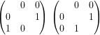
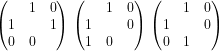
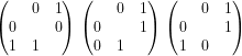
Survey of Animated Logical Graphs • 1

This is one of several Survey posts I’ll be drafting from time to time, starting with minimal stubs and collecting links to the better variations on persistent themes I’ve worked on over the years.  After that I’ll look to organizing and revising the assembled material with an eye toward developing more polished articles.

Elements

Excursions

Applications

Blog Dialogs

Posted in Abstraction, Amphecks, Animata, Boole, Boolean Algebra, Boolean Functions, C.S. Peirce, Cactus Graphs, Computational Complexity, Constraint Satisfaction Problems, Equational Inference, Graph Theory, Laws of Form, Logic, Logical Graphs, Mathematics, Minimal Negation Operators, Painted Cacti, Peirce, Propositional Calculus, Propositional Equation Reasoning Systems, Spencer Brown, Surveys, Theorem Proving, Visualization, Zeroth Order Logic | Tagged , , , , , , , , , , , , , , , , , , , , , , , , , | 2 Comments

Peirce’s 1880 “Algebra Of Logic” Chapter 3 • Comment 7.5

Suppose we add another individual to our initial universe of discourse, arriving at a three-point universe \{ \mathrm{I}, \mathrm{J}, \mathrm{K} \}.

It might be thought that adding one more element to the universe of discourse would allow slightly more complicated relations to be compounded from its basic ingredients, but the truth is that crossing the threshold from a two-point universe to a three-point universe occasions a steep ascent in the complexity of relations generated.

Looking back from the ascent we see that the two-point universe \{ \mathrm{I}, \mathrm{J} \} manifests a type of formal degeneracy (loss of generality) compared with the three-point universe \{ \mathrm{I}, \mathrm{J}, \mathrm{K} \}.  This is due to the circumstance that the number of “diagonal” pairs, those of the form \mathrm{A\!:\!A}, equals the number of “off-diagonal” pairs, those of the form \mathrm{A\!:\!B}, so the two-point case exhibits symmetries that will be broken as soon as one adds another element to the universe.

A universe of three individuals \mathrm{I, J, K} yields exactly nine individual dual relatives or ordered pairs of universe elements:

\begin{matrix}  \mathrm{I\!:\!I}, & \mathrm{I\!:\!J}, & \mathrm{I\!:\!K}, & \mathrm{J\!:\!I}, & \mathrm{J\!:\!J}, & \mathrm{J\!:\!K}, & \mathrm{K\!:\!I}, & \mathrm{K\!:\!J}, & \mathrm{K\!:\!K}.  \end{matrix}

It is convenient arrange the pairs in a square array:

\left( \begin{matrix}  \mathrm{I\!:\!I} & \mathrm{I\!:\!J} & \mathrm{I\!:\!K}  \\[4pt]  \mathrm{J\!:\!I} & \mathrm{J\!:\!J} & \mathrm{J\!:\!K}  \\[4pt]  \mathrm{K\!:\!I} & \mathrm{K\!:\!J} & \mathrm{K\!:\!K}  \end{matrix} \right)

There are 2^9 = 512 dual relatives over this universe of discourse, since each one is formed by choosing a subset of the nine ordered pairs and then “aggregating” them, forming their logical sum, or simply regarding them as a subset.  Taking the square array of ordered pairs as a backdrop, any one of the 512 dual relatives may be represented by a square matrix of binary values, a value of 1 occupying the place of each ordered pair that belongs to the subset and a value of 0 occupying the place of each ordered pair that does not belong to the subset in question.

The matrix representations of the 512 dual relatives or dyadic relations over the universe \{ \mathrm{I}, \mathrm{J}, \mathrm{K} \} are tabulated below according to the following plan:

  • Since the diagonal and off-diagonal components of the matrices vary independently of each other, the whole set of matrices factors as a product of two smaller sets, making the break along the lines of the corresponding cardinalities, 2^9 = 2^3 \times 2^6.
  • The eight diagonal matrices are shown in the first row of the display, omitting the off-diagonal zeroes for ease of reading and pattern recognition.
  • The 64 off-diagonal matrices are shown in the rest of the display, arranged in rank order by increasing numbers of \text{1's} and decreasing numbers of \text{0's}, suppressing the fixed zeroes along the diagonals to make the changing patterns of \text{0's} and \text{1's} easier to follow.
  • The number of off-diagonal matrices of rank k is equal to the binomial coefficient \tbinom{6}{k} or \mathrm{C}(6, k).  The values of \mathrm{C}(6, k)  are given by the row of Pascal’s Triangle that contains the sequence {1, 6, 15, 20, 15, 6, 1}.

\begin{pmatrix}  0 & ~ & ~ \\  ~ & 0 & ~ \\  ~ & ~ & 0  \end{pmatrix}  \,  \begin{pmatrix}  1 & ~ & ~ \\  ~ & 0 & ~ \\  ~ & ~ & 0  \end{pmatrix}  \,  \begin{pmatrix}  0 & ~ & ~ \\  ~ & 1 & ~ \\  ~ & ~ & 0  \end{pmatrix}  \,  \begin{pmatrix}  0 & ~ & ~ \\  ~ & 0 & ~ \\  ~ & ~ & 1  \end{pmatrix}  \,  \begin{pmatrix}  1 & ~ & ~ \\  ~ & 1 & ~ \\  ~ & ~ & 0  \end{pmatrix}  \,  \begin{pmatrix}  1 & ~ & ~ \\  ~ & 0 & ~ \\  ~ & ~ & 1  \end{pmatrix}  \,  \begin{pmatrix}  0 & ~ & ~ \\  ~ & 1 & ~ \\  ~ & ~ & 1  \end{pmatrix}  \,  \begin{pmatrix}  1 & ~ & ~ \\  ~ & 1 & ~ \\  ~ & ~ & 1  \end{pmatrix}

\times

\begin{pmatrix}  ~ & 0 & 0 \\  0 & ~ & 0 \\  0 & 0 & ~  \end{pmatrix}

\begin{pmatrix}  ~ & 1 & 0 \\  0 & ~ & 0 \\  0 & 0 & ~  \end{pmatrix}  \,  \begin{pmatrix}  ~ & 0 & 1 \\  0 & ~ & 0 \\  0 & 0 & ~  \end{pmatrix}  \,  \begin{pmatrix}  ~ & 0 & 0 \\  1 & ~ & 0 \\  0 & 0 & ~  \end{pmatrix}  \,  \begin{pmatrix}  ~ & 0 & 0 \\  0 & ~ & 1 \\  0 & 0 & ~  \end{pmatrix}  \,  \begin{pmatrix}  ~ & 0 & 0 \\  0 & ~ & 0 \\  1 & 0 & ~  \end{pmatrix}  \,  \begin{pmatrix}  ~ & 0 & 0 \\  0 & ~ & 0 \\  0 & 1 & ~  \end{pmatrix}

\begin{pmatrix}  ~ & 1 & 1 \\  0 & ~ & 0 \\  0 & 0 & ~  \end{pmatrix}  \,  \begin{pmatrix}  ~ & 1 & 0 \\  1 & ~ & 0 \\  0 & 0 & ~  \end{pmatrix}  \,  \begin{pmatrix}  ~ & 1 & 0 \\  0 & ~ & 1 \\  0 & 0 & ~  \end{pmatrix}  \,  \begin{pmatrix}  ~ & 1 & 0 \\  0 & ~ & 0 \\  1 & 0 & ~  \end{pmatrix}  \,  \begin{pmatrix}  ~ & 1 & 0 \\  0 & ~ & 0 \\  0 & 1 & ~  \end{pmatrix}

\begin{pmatrix}  ~ & 0 & 1 \\  1 & ~ & 0 \\  0 & 0 & ~  \end{pmatrix}  \,  \begin{pmatrix}  ~ & 0 & 1 \\  0 & ~ & 1 \\  0 & 0 & ~  \end{pmatrix}  \,  \begin{pmatrix}  ~ & 0 & 1 \\  0 & ~ & 0 \\  1 & 0 & ~  \end{pmatrix}  \,  \begin{pmatrix}  ~ & 0 & 1 \\  0 & ~ & 0 \\  0 & 1 & ~  \end{pmatrix}

\begin{pmatrix}  ~ & 0 & 0 \\  1 & ~ & 1 \\  0 & 0 & ~  \end{pmatrix}  \,  \begin{pmatrix}  ~ & 0 & 0 \\  1 & ~ & 0 \\  1 & 0 & ~  \end{pmatrix}  \,  \begin{pmatrix}  ~ & 0 & 0 \\  1 & ~ & 0 \\  0 & 1 & ~  \end{pmatrix}

\begin{pmatrix}  ~ & 0 & 0 \\  0 & ~ & 1 \\  1 & 0 & ~  \end{pmatrix}  \,  \begin{pmatrix}  ~ & 0 & 0 \\  0 & ~ & 1 \\  0 & 1 & ~  \end{pmatrix}

\begin{pmatrix}  ~ & 0 & 0 \\  0 & ~ & 0 \\  1 & 1 & ~  \end{pmatrix}

\begin{pmatrix}  ~ & 1 & 1 \\  1 & ~ & 0 \\  0 & 0 & ~  \end{pmatrix}  \,  \begin{pmatrix}  ~ & 1 & 1 \\  0 & ~ & 1 \\  0 & 0 & ~  \end{pmatrix}  \,  \begin{pmatrix}  ~ & 1 & 1 \\  0 & ~ & 0 \\  1 & 0 & ~  \end{pmatrix}  \,  \begin{pmatrix}  ~ & 1 & 1 \\  0 & ~ & 0 \\  0 & 1 & ~  \end{pmatrix}

\begin{pmatrix}  ~ & 1 & 0 \\  1 & ~ & 1 \\  0 & 0 & ~  \end{pmatrix}  \,  \begin{pmatrix}  ~ & 1 & 0 \\  1 & ~ & 0 \\  1 & 0 & ~  \end{pmatrix}  \,  \begin{pmatrix}  ~ & 1 & 0 \\  1 & ~ & 0 \\  0 & 1 & ~  \end{pmatrix}

\begin{pmatrix}  ~ & 1 & 0 \\  0 & ~ & 1 \\  1 & 0 & ~  \end{pmatrix}  \,  \begin{pmatrix}  ~ & 1 & 0 \\  0 & ~ & 1 \\  0 & 1 & ~  \end{pmatrix}

\begin{pmatrix}  ~ & 1 & 0 \\  0 & ~ & 0 \\  1 & 1 & ~  \end{pmatrix}

\begin{pmatrix}  ~ & 0 & 1 \\  1 & ~ & 1 \\  0 & 0 & ~  \end{pmatrix}

\begin{pmatrix}  ~ & 0 & 1 \\  1 & ~ & 0 \\  0 & 1 & ~  \end{pmatrix}  \,  \begin{pmatrix}  ~ & 0 & 1 \\  1 & ~ & 0 \\  1 & 0 & ~  \end{pmatrix}

\begin{pmatrix}  ~ & 0 & 1 \\  0 & ~ & 0 \\  1 & 1 & ~  \end{pmatrix}  \,  \begin{pmatrix}  ~ & 0 & 1 \\  0 & ~ & 1 \\  0 & 1 & ~  \end{pmatrix}  \,  \begin{pmatrix}  ~ & 0 & 1 \\  0 & ~ & 1 \\  1 & 0 & ~  \end{pmatrix}

\begin{pmatrix}  ~ & 0 & 0 \\  0 & ~ & 1 \\  1 & 1 & ~  \end{pmatrix}  \,  \begin{pmatrix}  ~ & 0 & 0 \\  1 & ~ & 0 \\  1 & 1 & ~  \end{pmatrix}  \,  \begin{pmatrix}  ~ & 0 & 0 \\  1 & ~ & 1 \\  0 & 1 & ~  \end{pmatrix}  \,  \begin{pmatrix}  ~ & 0 & 0 \\  1 & ~ & 1 \\  1 & 0 & ~  \end{pmatrix}

\begin{pmatrix}  ~ & 1 & 1 \\  1 & ~ & 1 \\  0 & 0 & ~  \end{pmatrix}

\begin{pmatrix}  ~ & 1 & 1 \\  1 & ~ & 0 \\  0 & 1 & ~  \end{pmatrix}  \,  \begin{pmatrix}  ~ & 1 & 1 \\  1 & ~ & 0 \\  1 & 0 & ~  \end{pmatrix}

\begin{pmatrix}  ~ & 1 & 1 \\  0 & ~ & 0 \\  1 & 1 & ~  \end{pmatrix}  \,  \begin{pmatrix}  ~ & 1 & 1 \\  0 & ~ & 1 \\  0 & 1 & ~  \end{pmatrix}  \,  \begin{pmatrix}  ~ & 1 & 1 \\  0 & ~ & 1 \\  1 & 0 & ~  \end{pmatrix}

\begin{pmatrix}  ~ & 1 & 0 \\  0 & ~ & 1 \\  1 & 1 & ~  \end{pmatrix}  \,  \begin{pmatrix}  ~ & 1 & 0 \\  1 & ~ & 0 \\  1 & 1 & ~  \end{pmatrix}  \,  \begin{pmatrix}  ~ & 1 & 0 \\  1 & ~ & 1 \\  0 & 1 & ~  \end{pmatrix}  \,  \begin{pmatrix}  ~ & 1 & 0 \\  1 & ~ & 1 \\  1 & 0 & ~  \end{pmatrix}

\begin{pmatrix}  ~ & 0 & 0 \\  1 & ~ & 1 \\  1 & 1 & ~  \end{pmatrix}  \,  \begin{pmatrix}  ~ & 0 & 1 \\  0 & ~ & 1 \\  1 & 1 & ~  \end{pmatrix}  \,  \begin{pmatrix}  ~ & 0 & 1 \\  1 & ~ & 0 \\  1 & 1 & ~  \end{pmatrix}  \,  \begin{pmatrix}  ~ & 0 & 1 \\  1 & ~ & 1 \\  0 & 1 & ~  \end{pmatrix}  \,  \begin{pmatrix}  ~ & 0 & 1 \\  1 & ~ & 1 \\  1 & 0 & ~  \end{pmatrix}

\begin{pmatrix}  ~ & 0 & 1 \\  1 & ~ & 1 \\  1 & 1 & ~  \end{pmatrix}  \,  \begin{pmatrix}  ~ & 1 & 0 \\  1 & ~ & 1 \\  1 & 1 & ~  \end{pmatrix}  \,  \begin{pmatrix}  ~ & 1 & 1 \\  0 & ~ & 1 \\  1 & 1 & ~  \end{pmatrix}  \,  \begin{pmatrix}  ~ & 1 & 1 \\  1 & ~ & 0 \\  1 & 1 & ~  \end{pmatrix}  \,  \begin{pmatrix}  ~ & 1 & 1 \\  1 & ~ & 1 \\  0 & 1 & ~  \end{pmatrix}  \,  \begin{pmatrix}  ~ & 1 & 1 \\  1 & ~ & 1 \\  1 & 0 & ~  \end{pmatrix}

\begin{pmatrix}  ~ & 1 & 1 \\  1 & ~ & 1 \\  1 & 1 & ~  \end{pmatrix}

References

  • Peirce, C.S. (1880), “On the Algebra of Logic”, American Journal of Mathematics 3, 15–57.  Collected Papers (CP 3.154–251), Chronological Edition (CE 4, 163–209).
  • Peirce, C.S., Collected Papers of Charles Sanders Peirce, vols. 1–6, Charles Hartshorne and Paul Weiss (eds.), vols. 7–8, Arthur W. Burks (ed.), Harvard University Press, Cambridge, MA, 1931–1935, 1958.  Volume 3 : Exact Logic, 1933.
  • Peirce, C.S., Writings of Charles S. Peirce : A Chronological Edition, Peirce Edition Project (eds.), Indiana University Press, Bloomington and Indianapolis, IN, 1981–.  Volume 4 (1879–1884), 1986.

Resources

Posted in Dyadic Relations, Graph Theory, Logic, Logic of Relatives, Mathematics, Matrix Theory, Peirce, Relation Theory, Semiotics, Sign Relations, Triadic Relations | Tagged , , , , , , , , , , | 10 Comments

Peirce’s 1880 “Algebra Of Logic” Chapter 3 • Comment 7.4

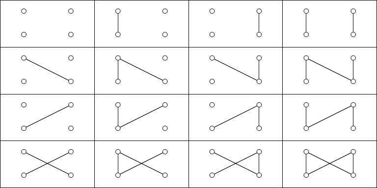
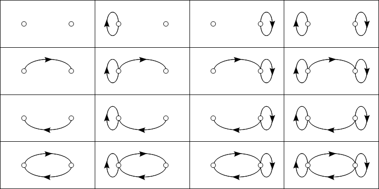
Dyadic relations enjoy yet another form of graph-theoretic representation as labeled bipartite graphs or labeled bigraphs.  I’ll just call them bigraphs here, letting the labels be understood in this logical context.

The figure below shows the bigraphs of the 16 dyadic relations on two points, adopting the same arrangement as the previous displays of binary matrices and loopy digraphs.

Dyadic Relation Bigraphs 2 Points

References

  • Peirce, C.S. (1880), “On the Algebra of Logic”, American Journal of Mathematics 3, 15–57.  Collected Papers (CP 3.154–251), Chronological Edition (CE 4, 163–209).
  • Peirce, C.S., Collected Papers of Charles Sanders Peirce, vols. 1–6, Charles Hartshorne and Paul Weiss (eds.), vols. 7–8, Arthur W. Burks (ed.), Harvard University Press, Cambridge, MA, 1931–1935, 1958.  Volume 3 : Exact Logic, 1933.
  • Peirce, C.S., Writings of Charles S. Peirce : A Chronological Edition, Peirce Edition Project (eds.), Indiana University Press, Bloomington and Indianapolis, IN, 1981–.  Volume 4 (1879–1884), 1986.

Resources

Posted in Dyadic Relations, Graph Theory, Logic, Logic of Relatives, Mathematics, Matrix Theory, Peirce, Relation Theory, Semiotics, Sign Relations, Triadic Relations | Tagged , , , , , , , , , , | 9 Comments

Peirce’s 1880 “Algebra Of Logic” Chapter 3 • Comment 7.3

Dyadic relations have graph-theoretic representations as labeled directed graphs with loops, also known as labeled pseudo-digraphs in some schools of graph theory.  I’ll just call them digraphs here, letting the labels and loops be understood in this logical context.

The figure below shows the digraphs of the 16 dyadic relations on two points, adopting the same arrangement as the previous display of binary matrices.

Dyadic Relations 2 Points

References

  • Peirce, C.S. (1880), “On the Algebra of Logic”, American Journal of Mathematics 3, 15–57.  Collected Papers (CP 3.154–251), Chronological Edition (CE 4, 163–209).
  • Peirce, C.S., Collected Papers of Charles Sanders Peirce, vols. 1–6, Charles Hartshorne and Paul Weiss (eds.), vols. 7–8, Arthur W. Burks (ed.), Harvard University Press, Cambridge, MA, 1931–1935, 1958.  Volume 3 : Exact Logic, 1933.
  • Peirce, C.S., Writings of Charles S. Peirce : A Chronological Edition, Peirce Edition Project (eds.), Indiana University Press, Bloomington and Indianapolis, IN, 1981–.  Volume 4 (1879–1884), 1986.

Resources

Posted in Dyadic Relations, Graph Theory, Logic, Logic of Relatives, Mathematics, Matrix Theory, Peirce, Relation Theory, Semiotics, Sign Relations, Triadic Relations | Tagged , , , , , , , , , , | 10 Comments

Peirce’s 1880 “Algebra Of Logic” Chapter 3 • Comment 7.2

Because it can sometimes be difficult to reconnect abstractions with their concrete instances, especially after the abstract types have become autonomous and taken on a life of their own, let us resort to a simple concrete case and examine the implications of what Peirce is saying about the relation between general relatives and individual relatives.

Suppose our initial universe of discourse has exactly two individuals, \mathrm{I} and \mathrm{J}.  Then there are exactly four individual dual relatives or ordered pairs of universe elements:

\begin{matrix}  \mathrm{I\!:\!I}, & \mathrm{I\!:\!J}, & \mathrm{J\!:\!I}, & \mathrm{J\!:\!J}.  \end{matrix}

It is convenient arrange these in a square array:

\left( \begin{array}{rr}  \mathrm{I\!:\!I} & \mathrm{I\!:\!J} \\[4pt]  \mathrm{J\!:\!I} & \mathrm{J\!:\!J}  \end{array} \right)

There are 2^4 = 16 dual relatives in general over this universe of discourse, since each one is formed by choosing a subset of the four ordered pairs and then “aggregating” them, forming their logical sum, or simply regarding them as a subset.  Taking the square array of ordered pairs as a backdrop, any one of the 16 dual relatives may be represented by a square matrix of binary values, a value of 1 occupying the place of each ordered pair that belongs to the subset and a value of 0 occupying the place of each ordered pair that does not belong to the subset in question.  The matrix representations of the 16 dual relatives or dyadic relations over the universe \{ \mathrm{I}, \mathrm{J} \} are displayed below:

\begin{pmatrix}  0 & 0 \\  0 & 0  \end{pmatrix}  \quad  \begin{pmatrix}  1 & 0 \\  0 & 0  \end{pmatrix}  \quad  \begin{pmatrix}  0 & 0 \\  0 & 1  \end{pmatrix}  \quad  \begin{pmatrix}  1 & 0 \\  0 & 1  \end{pmatrix}

\begin{pmatrix}  0 & 1 \\  0 & 0  \end{pmatrix}  \quad  \begin{pmatrix}  1 & 1 \\  0 & 0  \end{pmatrix}  \quad  \begin{pmatrix}  0 & 1 \\  0 & 1  \end{pmatrix}  \quad  \begin{pmatrix}  1 & 1 \\  0 & 1  \end{pmatrix}

\begin{pmatrix}  0 & 0 \\  1 & 0  \end{pmatrix}  \quad  \begin{pmatrix}  1 & 0 \\  1 & 0  \end{pmatrix}  \quad  \begin{pmatrix}  0 & 0 \\  1 & 1  \end{pmatrix}  \quad  \begin{pmatrix}  1 & 0 \\  1 & 1  \end{pmatrix}

\begin{pmatrix}  0 & 1 \\  1 & 0  \end{pmatrix}  \quad  \begin{pmatrix}  1 & 1 \\  1 & 0  \end{pmatrix}  \quad  \begin{pmatrix}  0 & 1 \\  1 & 1  \end{pmatrix}  \quad  \begin{pmatrix}  1 & 1 \\  1 & 1  \end{pmatrix}

Relative to the universe \{ \mathrm{I}, \mathrm{J} \}, the individual dual relatives of the form \mathrm{A\!:\!A} are \mathrm{I\!:\!I} and \mathrm{J\!:\!J} while the individual dual relatives of the form \mathrm{A\!:\!B} are \mathrm{I\!:\!J} and \mathrm{J\!:\!I}.

Peirce assigns the name concurrents to dual relatives all whose individual aggregants are of the form \mathrm{A\!:\!A}.  There are exactly 4 of these and their matrices are shown in the top row of the above display.  All the rest are called opponents and their matrices are listed in the bottom three rows.

Peirce gives the name alio-relatives to dual relatives all whose individual aggregants are of the form \mathrm{A\!:\!B}.  There are exactly 4 of these and their matrices are shown in the first column of the above display.  All the rest are called self-relatives and their matrices are listed in the right hand three columns.

Notice that the relative {0}, represented by the matrix with all {0} entries, falls under the definitions of both a concurrent and an alio-relative.

References

  • Peirce, C.S. (1880), “On the Algebra of Logic”, American Journal of Mathematics 3, 15–57.  Collected Papers (CP 3.154–251), Chronological Edition (CE 4, 163–209).
  • Peirce, C.S., Collected Papers of Charles Sanders Peirce, vols. 1–6, Charles Hartshorne and Paul Weiss (eds.), vols. 7–8, Arthur W. Burks (ed.), Harvard University Press, Cambridge, MA, 1931–1935, 1958.  Volume 3 : Exact Logic, 1933.
  • Peirce, C.S., Writings of Charles S. Peirce : A Chronological Edition, Peirce Edition Project (eds.), Indiana University Press, Bloomington and Indianapolis, IN, 1981–.  Volume 4 (1879–1884), 1986.

Resources

Posted in Dyadic Relations, Logic, Logic of Relatives, Mathematics, Matrix Theory, Peirce, Relation Theory, Semiotics, Sign Relations, Triadic Relations | Tagged , , , , , , , , , | 11 Comments

Peirce’s 1880 “Algebra Of Logic” Chapter 3 • Comment 7.1

I wanted to call attention to a very important statement from Selection 7 (CP 3.225–226).  Peirce enumerates the fundamental forms of individual dual relatives in the following terms:

225.   Individual relatives are of one or other of the two forms

\begin{array}{lll}  \mathrm{A : A} & \qquad & \mathrm{A : B},  \end{array}

and simple relatives are negatives of one or other of these two forms.

And then he makes the following observation:

226.   The forms of general relatives are of infinite variety, but the following may be particularly noticed.

Relatives may be divided into those all whose individual aggregants are of the form \mathrm{A : A} and those which contain individuals of the form \mathrm{A : B}.  The former may be called concurrents, the latter opponents.

This tells us that Peirce understands the distinction between general dual relatives and individual dual relatives, the individuals being “aggregated” or logically summed to form the generals, and that singling out special cases of general relatives in the way he does next is but a first rough cut toward a complete classification.  This needs to be born in mind as we proceed toward the enumeration of triadic relations and beyond, especially as it affects the classification of triadic sign relations.

References

  • Peirce, C.S. (1880), “On the Algebra of Logic”, American Journal of Mathematics 3, 15–57.  Collected Papers (CP 3.154–251), Chronological Edition (CE 4, 163–209).
  • Peirce, C.S., Collected Papers of Charles Sanders Peirce, vols. 1–6, Charles Hartshorne and Paul Weiss (eds.), vols. 7–8, Arthur W. Burks (ed.), Harvard University Press, Cambridge, MA, 1931–1935, 1958.  Volume 3 : Exact Logic, 1933.
  • Peirce, C.S., Writings of Charles S. Peirce : A Chronological Edition, Peirce Edition Project (eds.), Indiana University Press, Bloomington and Indianapolis, IN, 1981–.  Volume 4 (1879–1884), 1986.

Resources

Posted in Dyadic Relations, Logic, Logic of Relatives, Mathematics, Peirce, Relation Theory, Semiotics, Sign Relations, Triadic Relations | Tagged , , , , , , , , | 9 Comments

Objective Frameworks • Properties and Instances 1

Dealing with sign relations containing many types of signs — icons, indices, symbols, and more complex varieties — calls for a flexible and powerful organizational framework, one with the ability to grow and develop over time.  This is one of those applications where I found it useful to consider a “relative membership” relation, adding a parameter for the interpreter to the ordinary set-theoretic membership.

I laid out the details of a formalization in the following paragraphs:

It begins as follows:

In accounting for the special characters of icons and indices that arose in previous discussions, it was necessary to open the domain of objects coming under formal consideration to include unspecified numbers of properties and instances of whatever objects were initially set down.  This is a general phenomenon, affecting every motion toward explanation whether pursued by analytic or synthetic means.  What it calls for in practice is a way of organizing growing domains of objects, without having to specify in advance all the objects there are.

Posted in C.S. Peirce, Icon Index Symbol, Inquiry, Interpretive Frameworks, Logic, Logic of Relatives, Mathematics, Objective Frameworks, Peirce, Relation Theory, Relative Membership, Semiotics, Set Theory, Sign Relations | Tagged , , , , , , , , , , , , , | 2 Comments

Relations & Their Relatives • Discussion 5

Re: Peirce List • Howard Pattee

At this point we can distinguish two forms of decomposability or reducibility — along with their corresponding negations, indecomposability or irreducibility – that commonly arise.

  • Reducibility under relational composition P \circ Q.

All triadic relations are irreducible in this sense.  This is because relational compositions of monadic and dyadic relations can produce only more monadic and dyadic relations.

  • Reducibility under projections.  For this we need a few definitions:

Every triadic relation, say L contained as a subset of the cartesian product X \times Y \times Z, determines three dyadic relations, namely, the projections of L on the three “planes” X \times Y, X \times Z, and Y \times Z.

In particular:

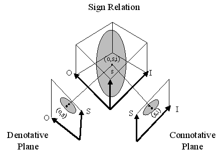
Every sign relation, say M contained as a subset of the cartesian product O \times S \times I, those being the sets of objects, signs, and interpretant signs respectively under discussion, determines three dyadic relations, which we may notate as follows:

  • \mathrm{proj}_{OS}{M}, the projection of M on the O \times S plane;
  • \mathrm{proj}_{OI}{M}, the projection of M on the O \times I plane;
  • \mathrm{proj}_{SI}{M}, the projection of M on the S \times I plane.

The following Figure illustrates the situation.

Aspects of a Sign Relation

Here is the critical point.  The triadic relation always determines the three dyadic projections but the three dyadic projections may or may not determine the triadic relation.  Thus we have two cases:

  • If the dyadic projections determine the triadic relation, that is, there is only one triadic relation that has those three projections, then the triadic relation is said to be projectively reducible to those three dyadic relations.
  • If the dyadic projections do not determine the triadic relation, that is, there is more than one triadic relation that has those same three projections, then the triadic relation is said to be projectively irreducible.

See the following article for concrete examples of both possibilities, a pair of generic triadic relations that are projectively irreducible and a pair of triadic sign relations that are projectively reducible to their dyadic projections.

Resources

Posted in C.S. Peirce, Category Theory, Control, Cybernetics, Dyadic Relations, Information, Inquiry, Logic, Logic of Relatives, Mathematics, Peirce, Relation Theory, Semiosis, Semiotics, Sign Relations, Systems Theory, Triadic Relations | Tagged , , , , , , , , , , , , , , , , | 15 Comments

Relations & Their Relatives • Discussion 4

Re: Peirce List Discussion • Howard Pattee

We use this or that species of diagrams to represent a fraction of the properties, hardly ever all the properties, of the objects in an object domain.  The diagrams that Peirce developed to represent propositions about relations are quite handy so long as one grasps the conventions of representation, manipulation, and interpretation.  They are not all that different in kind from Feynman interaction diagrams or Penrose twistor diagrams.  Iconicity is nice when you can get it but one has to keep in mind that the map is not the territory, as the saying goes.

What do I see in a picture like this?

         s  
        /   
  o---<L    
        \   
         i  

The ``L" brings to mind a triadic relation L, which collateral knowledge tells me is a set of triples.  What sort of triples?  The picture sets a place for them by means of the place-names ``o", ``s", ``i", in no particular order.  Without loss of generality I can take them up in the ordered triple (o, s, i).  All of this is just mnemonic machination meant to say that a typical element is (o, s, i) in L.  It’s up to me to remember that L is a subset of O \times S \times I, with o \in O, s \in S, and i \in I.  The diagram is just a mnemonic catalyst.  You have to know the codebook to decode it.

Pictures can victimize people, as Wittgenstein remarked and often exemplified.  One way people fall victim to pictures like the one depicted above is when they confuse a relation with a single one of its tuples.  That would represent a misunderstanding of what the picture is intended to represent.

Resources

Posted in Diagrammatic Reasoning, Diagrams, Logic, Logic of Relatives, Mathematics, Peirce, Peirce List, Relation Theory, Semiotics, Sign Relations, Tertium Quid, Thirdness, Triadic Relations, Triadicity | Tagged , , , , , , , , , , , , , | 12 Comments

Animated Logical Graphs • 6

Re: Peirce List • Jim Willgoose

At root we are dealing with a genre of very abstract formal systems.  They have grammars that determine their well-formed expressions and rules that determine the permissible transformations among expressions, but they lack all logical meaning until we supply an interpretation.

The formal system Peirce developed for propositional logic and Spencer Brown resurrected for his Laws of Form admits a formal duality which allows it to be fleshed out with logical meanings in two distinct ways.  The two interpretations are employed in Peirce’s entitative graphs and existential graphs, respectively.  It is clear from everything they write that both authors are well aware of both interpretations, but Peirce would come to found his later developments on the existential sense while Spencer Brown favored the entitative sense in his expositions.

See the following readings for further discussion.

References

Posted in Amphecks, Analogy, Animata, Automated Research Tools, Boolean Algebra, Boolean Functions, C.S. Peirce, Cactus Graphs, Constraint Satisfaction Problems, Deduction, Diagrammatic Reasoning, Duality, Graph Theory, Iconicity, Laws of Form, Logic, Logical Graphs, Mathematics, Model Theory, Peirce, Peirce's Law, Praeclarum Theorema, Pragmatism, Proof Theory, Propositional Calculus, Semiotics, Spencer Brown, Theorem Proving, Visualization | Tagged , , , , , , , , , , , , , , , , , , , , , , , , , , , , | 12 Comments