Moving Pictures of Thought
A logical graph is a graph‑theoretic structure in one of the systems of graphical syntax Charles S. Peirce developed for logic.
Introduction
In numerous papers on qualitative logic, entitative graphs, and existential graphs, Peirce developed several versions of a graphical formalism, or a graph‑theoretic formal language, designed to be interpreted for logic.
In the century since Peirce initiated this line of development, a variety of formal systems have branched out from what is abstractly the same formal base of graph-theoretic structures. This article examines the common basis of this class of formal systems from a bird’s eye view, focusing on the aspects of form shared by the entire family of algebras, calculi, or languages, however they happen to be viewed in a given application.
Abstract Point of View
The bird’s eye view in question is more formally known as the perspective of formal equivalence, from which remove one overlooks many distinctions that appear momentous in more concrete settings. Expressions inscribed in different formalisms whose syntactic structures are algebraically or topologically isomorphic are not recognized as being different from each other in any significant sense. An eye to historical detail will note in passing that C.S. Peirce used a streamer-cross symbol where Spencer Brown used a carpenter’s square marker to roughly the same formal purpose, for instance, but the main theme of interest at the level of pure form is indifferent to variations of that order.
In Lieu of a Beginning
Consider the following two formal equations.
 |
(1) |
 |
(2) |
Duality : Logical and Topological
In using logical graphs there are two types of duality to consider, logical duality and topological duality.
Graphs of the order Peirce considered, those embedded in a continuous manifold like that commonly represented by a plane sheet of paper, can be represented in linear text as what are called traversal strings and parsed into pointer structures in computer memory.
A blank sheet of paper can be represented in linear text as a blank space, but that way of doing it tends to be confusing unless the logical expression under consideration is set off in a separate display.
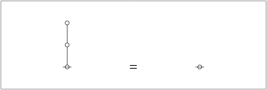
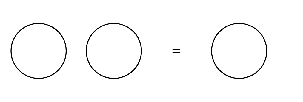
For example, consider the axiom or initial equation shown below.
 |
(3) |
This can be written inline as “( ( ) ) = ” or set off in a text display:
( ( ) ) =
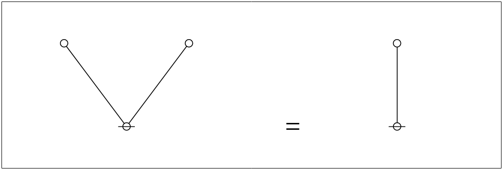
When we turn to representing the corresponding expressions in computer memory, where they can be manipulated with the greatest of ease, we begin by transforming the planar graphs into their topological duals. The planar regions of the original graph correspond to nodes (or points) of the dual graph, and the boundaries between planar regions in the original graph correspond to edges (or lines) between the nodes of the dual graph.
For example, overlaying the corresponding dual graphs on the plane-embedded graphs shown above, we get the following composite picture.
 |
(4) |
Though it’s not really there in the most abstract topology of the matter, for all sorts of pragmatic reasons we find ourselves compelled to single out the outermost region of the plane in a distinctive way and to mark it as the root node of the corresponding dual graph. In the present style of Figure the root nodes are marked by horizontal strike-throughs.
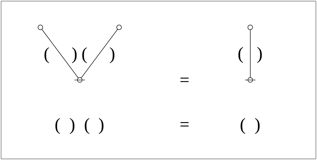
Extracting the dual graphs from their composite matrix, we get the following equation.
 |
(5) |
It is easy to see the relationship between the parenthetical representations of Peirce’s logical graphs, clippedly picturing the ordered containments of their formal contents, and the corresponding dual graphs, constituting a species of rooted trees to be described in greater detail below.
In the case of our last example, a moment’s contemplation of the following picture will lead us to see how we can get the corresponding parenthesis string by starting at the root of the tree, climbing up the left side of the tree until we reach the top, then climbing back down the right side of the tree until we return to the root, all the while reading off the symbols, in this case either “(” or “)”, we happen to encounter in our travels.
 |
(6) |
This ritual is called traversing the tree, and the string read off is often called the traversal string of the tree. The reverse ritual, which passes from the string to the tree, is called parsing the string, and the tree constructed is often called the parse graph of the string. The users of this jargon tend to use it loosely, often using parse string to mean the string that gets parsed into the associated graph.
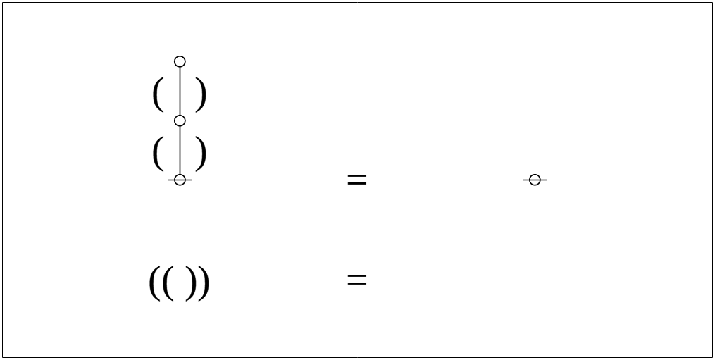
We have now treated in some detail various forms of the axiom or initial equation which is formulated in string form as “( ( ) ) = ”. For the sake of comparison, let’s record the planar and dual forms of the axiom which is formulated in string form as “( )( ) = ( )”.
First the plane-embedded maps:
 |
(7) |
Next the plane maps and their dual trees superimposed:
 |
(8) |
Finally the rooted trees by themselves:
 |
(9) |
And here are the parse trees with their traversal strings indicated:
 |
(10) |
We have at this point enough material to begin thinking about the forms of analogy, iconicity, metaphor, morphism, whatever we may call them, which bear on the use of logical graphs in their various incarnations, for example, those Peirce described as entitative graphs and existential graphs.
Computational Representation
The parse graphs we’ve been looking at so far bring us one step closer to the pointer graphs it takes to make the above types of maps and trees live in computer memory but they are still a couple of steps too abstract to detail the concrete species of dynamic data structures we need. The time has come to flesh out the skeletons we have drawn up to this point.
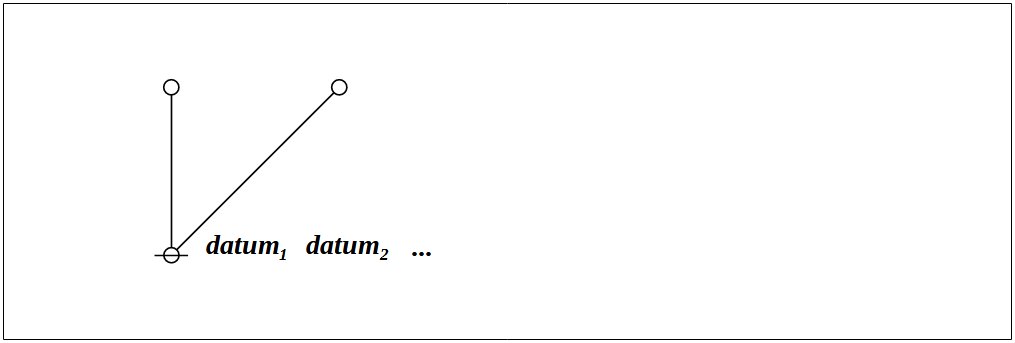
Nodes in a graph represent records in computer memory. A record is a collection of data which can be conceived to reside at a specific address. The address of a record is analogous to a demonstrative pronoun, a word like this or that, on which account programmers call it a pointer and semioticians recognize it as a type of sign called an index.
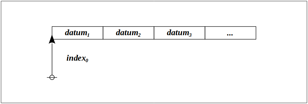
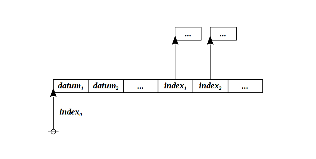
At the next level of concreteness, a pointer‑record data structure can be represented as follows.
 |
(11) |
This portrays index0 as the address of a record which contains the following data.
datum1, datum2, datum3, …, and so on.
What makes it possible to represent graph-theoretical structures as data structures in computer memory is the fact that an address is just another datum, and so we may have a state of affairs like the following.
 |
(12) |
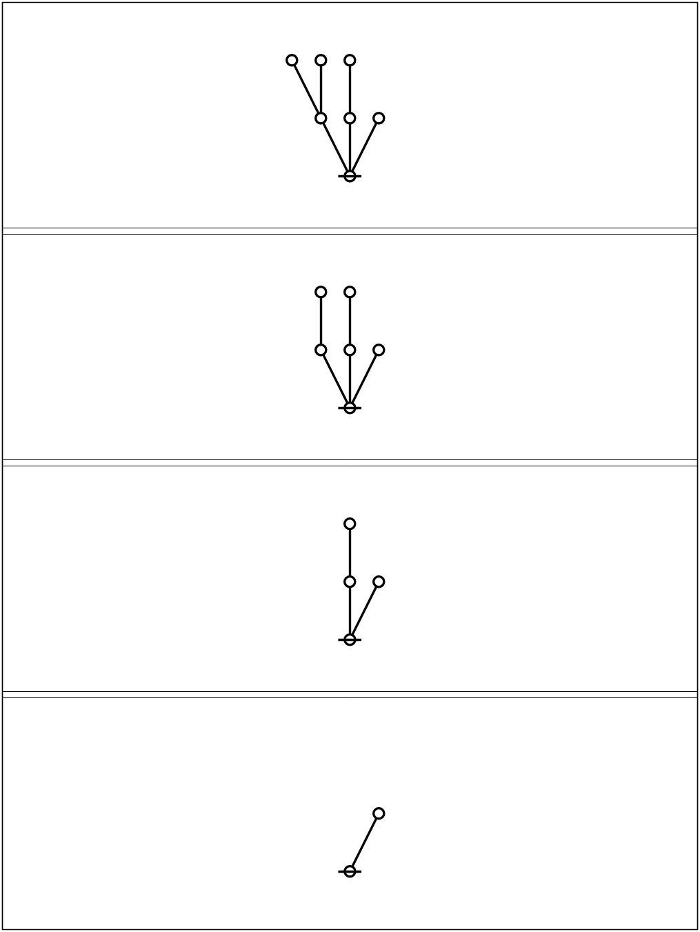
Returning to the abstract level, it takes three nodes to represent the three data records illustrated above: one root node connected to a couple of adjacent nodes. The items of data that do not point any further up the tree are then treated as labels on the record-nodes where they reside, as shown below.
 |
(13) |
Notice that drawing the arrows is optional with rooted trees like these, since singling out a unique node as the root induces a unique orientation on all the edges of the tree, with up being the same direction as away from the root.
Quick Tour of the Neighborhood
This much preparation allows us to take up the founding axioms or initial equations which determine the entire system of logical graphs.
Primary Arithmetic as Semiotic System
Though it may not seem too exciting, logically speaking, there are many reasons to make oneself at home with the system of forms represented indifferently, topologically speaking, by rooted trees, balanced strings of parentheses, and finite sets of non‑intersecting simple closed curves in the plane.
- For one thing it gives us a non‑trivial example of a sign domain on which to cut our semiotic teeth, non‑trivial in the sense that it contains a countable infinity of signs.
- In addition it allows us to study a simple form of computation recognizable as a species of semiosis or sign‑transforming process.
This space of forms, along with the pair of axioms which divide it into two formal equivalence classes, is what Spencer Brown called the primary arithmetic.
The axioms of the primary arithmetic are shown below, as they appear in both graph and string forms, along with pairs of names which come in handy for referring to the two opposing directions of applying the axioms.


Let  be the set of rooted trees and let
  be the 2‑element subset consisting of a rooted node and a rooted edge. Simple intuition, or a simple inductive proof, will assure us that any rooted tree can be reduced by means of the axioms of the primary arithmetic to either a root node or a rooted edge.
For example, consider the reduction which proceeds as follows.
 |
(16) |
Regarded as a semiotic process, this amounts to a sequence of signs, every one after the first serving as the interpretant of its predecessor, ending in a final sign which may be taken as the canonical sign for their common object, in the upshot being the result of the computation process. Simple as it is, this exhibits the main features of any computation, namely, a semiotic process proceeding from an obscure sign to a clear sign of the same object, being in its aim and effect an action on behalf of clarification.
Primary Algebra as Pattern Calculus
Experience teaches that complex objects are best approached in a gradual, laminar, modular fashion, one step, one layer, one piece at a time, especially when that complexity is irreducible, when all our articulations and all our representations will be cloven at joints disjoint from the structure of the object itself, with some assembly required in the synthetic integrity of the intuition.
That’s one good reason for spending so much time on the first half of zeroth order logic, represented here by the primary arithmetic, a level of formal structure Peirce verged on intuiting at numerous points and times in his work on logical graphs but Spencer Brown named and brought more completely to life.
Another reason for lingering a while longer in these primitive forests is that an acquaintance with “bare trees”, those unadorned with literal or numerical labels, will provide a basis for understanding what’s really at issue in oft‑debated questions about the “ontological status of variables”.
It is probably best to illustrate this theme in the setting of a concrete case. To do that let’s look again at the previous example of reductive evaluation taking place in the primary arithmetic.
|
(16) |
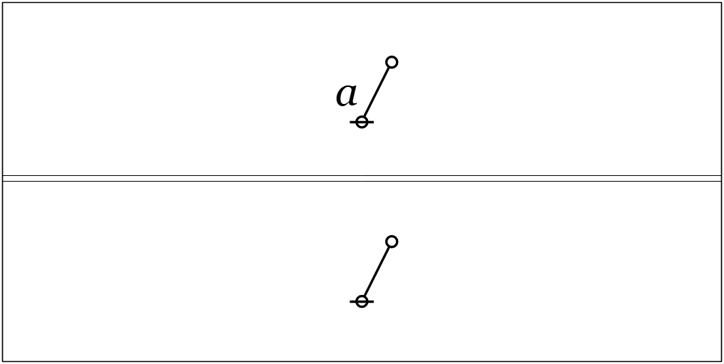
After we’ve seen a few sign-transformations of roughly that shape we’ll most likely notice it doesn’t really matter what other branches are rooted next to the lone edge off to the side — the end result will always be the same. Eventually it will occur to us to summarize the results of many such observations by introducing a label or variable to signify any shape of branch whatever, writing something like the following.
 |
(17) |
Observations like that, made about an arithmetic of any variety and germinated by their summarizations, are the root of all algebra.
Speaking of algebra, and having just encountered one example of an algebraic law, we might as well introduce the axioms of the primary algebra, once again deriving their substance and their name from the works of Charles Sanders Peirce and George Spencer Brown, respectively.


The choice of axioms for any formal system is to some degree a matter of aesthetics, as it is commonly the case that many different selections of formal rules will serve as axioms to derive all the rest as theorems. As it happens, the example of an algebraic law we noticed first, “a ( ) = ( )”, as simple as it appears, proves to be provable as a theorem on the grounds of the foregoing axioms.
We might also notice at this point a subtle difference between the primary arithmetic and the primary algebra with respect to the grounds of justification we have naturally if tacitly adopted for their respective sets of axioms.
The arithmetic axioms were introduced by fiat, in a quasi‑apriori fashion, though it is of course only long prior experience with the practical uses of comparably developed generations of formal systems that would actually induce us to such a quasi‑primal move. The algebraic axioms, in contrast, can be seen to derive both their motive and their justification from the observation and summarization of patterns which are visible in the arithmetic spectrum.
Formal Development
Discussion of the topic continues at Logical Graphs • Formal Development.
Resources
cc: FB | Logical Graphs • Laws of Form • Mathstodon • Academia.edu
cc: Conceptual Graphs • Cybernetics • Structural Modeling • Systems Science


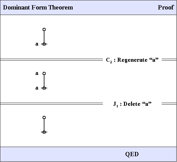
![\begin{array}{ccccc} \mathrm{I_1} & : & \text{true} ~ \text{or} ~ \text{true} & = & \text{true} \\[4pt] \mathrm{I_2} & : & \text{not} ~ \text{true} & = & \text{false} \\[4pt] \mathrm{J_1} & : & a ~ \text{or} ~ \text{not} ~ a & = & \text{true} \\[4pt] \mathrm{J_2} & : & (a ~ \text{or} ~ b) ~ \text{and} ~ (a ~ \text{or} ~ c) & = & a ~ \text{or} ~ (b ~ \text{and} ~ c) \end{array}](https://s0.wp.com/latex.php?latex=%5Cbegin%7Barray%7D%7Bccccc%7D++%5Cmathrm%7BI_1%7D++%26+%3A+%26+%5Ctext%7Btrue%7D+%7E+%5Ctext%7Bor%7D+%7E+%5Ctext%7Btrue%7D++%26+%3D+%26+%5Ctext%7Btrue%7D++%5C%5C%5B4pt%5D++%5Cmathrm%7BI_2%7D++%26+%3A+%26+%5Ctext%7Bnot%7D+%7E+%5Ctext%7Btrue%7D++%26+%3D+%26+%5Ctext%7Bfalse%7D++%5C%5C%5B4pt%5D++%5Cmathrm%7BJ_1%7D++%26+%3A+%26+a+%7E+%5Ctext%7Bor%7D+%7E+%5Ctext%7Bnot%7D+%7E+a++%26+%3D+%26+%5Ctext%7Btrue%7D++%5C%5C%5B4pt%5D++%5Cmathrm%7BJ_2%7D++%26+%3A+%26+%28a+%7E+%5Ctext%7Bor%7D+%7E+b%29+%7E+%5Ctext%7Band%7D+%7E+%28a+%7E+%5Ctext%7Bor%7D+%7E+c%29++%26+%3D+%26+a+%7E+%5Ctext%7Bor%7D+%7E+%28b+%7E+%5Ctext%7Band%7D+%7E+c%29++%5Cend%7Barray%7D&bg=ffffff&fg=000000&s=1&c=20201002)
![\begin{array}{ccccc} \mathrm{I_1} & : & \text{false} ~ \text{and} ~ \text{false} & = & \text{false} \\[4pt] \mathrm{I_2} & : & \text{not} ~ \text{false} & = & \text{true} \\[4pt] \mathrm{J_1} & : & a ~ \text{and} ~ \text{not} ~ a & = & \text{false} \\[4pt] \mathrm{J_2} & : & (a ~ \text{and} ~ b) ~ \text{or} ~ (a\ \text{and}\ c) & = & a ~ \text{and} ~ (b ~ \text{or} ~ c) \end{array}](https://s0.wp.com/latex.php?latex=%5Cbegin%7Barray%7D%7Bccccc%7D++%5Cmathrm%7BI_1%7D++%26+%3A+%26+%5Ctext%7Bfalse%7D+%7E+%5Ctext%7Band%7D+%7E+%5Ctext%7Bfalse%7D++%26+%3D+%26+%5Ctext%7Bfalse%7D++%5C%5C%5B4pt%5D++%5Cmathrm%7BI_2%7D++%26+%3A+%26+%5Ctext%7Bnot%7D+%7E+%5Ctext%7Bfalse%7D++%26+%3D+%26+%5Ctext%7Btrue%7D++%5C%5C%5B4pt%5D++%5Cmathrm%7BJ_1%7D++%26+%3A+%26+a+%7E+%5Ctext%7Band%7D+%7E+%5Ctext%7Bnot%7D+%7E+a+++%26+%3D+%26+%5Ctext%7Bfalse%7D++%5C%5C%5B4pt%5D++%5Cmathrm%7BJ_2%7D++%26+%3A+%26+%28a+%7E+%5Ctext%7Band%7D+%7E+b%29+%7E+%5Ctext%7Bor%7D+%7E+%28a%5C+%5Ctext%7Band%7D%5C+c%29++%26+%3D+%26+a+%7E+%5Ctext%7Band%7D+%7E+%28b+%7E+%5Ctext%7Bor%7D+%7E+c%29++%5Cend%7Barray%7D&bg=ffffff&fg=000000&s=1&c=20201002)
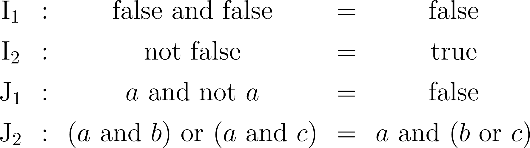
 have the form of equations. This means the inference steps they license are reversible. The proof annotation scheme employed below makes use of double bars
  to mark this fact, though it will often be left to the reader to decide which of the two possible directions is the one required for applying the indicated axiom.