Transfer
Returning to the scene of Dewey’s “Sign of Rain” example, let’s continue examining how the transfer of knowledge through the analogy of experience works in that case.
By way of a recap, we began by considering a fragment  of the reasoner’s knowledge base which is logically equivalent to a conjunction of two rules.

may be thought of as a piece of knowledge or item of information allowing for the possibility of certain conditions, expressed in the form of a logical constraint on the present universe of discourse.
Next we found it convenient to express all logical statements in terms of their models, that is, in terms of the primitive circumstances or elements of experience over which they hold true.
- Let
 be the chosen set of experiences, or the circumstances in mind under “past experience”.
- Let
 be the collective set of experiences, or the prospective total of possible circumstances.
- Let
 be the current experience, or the circumstances immediately present to the reasoner.
If we think of the knowledge base as referring to the “regime of experience” over which it is valid, then the sets of models involved in the analogy may be ordered according to the relationships of set inclusion or logical implication existing among them.
Figure 4 shows the subsumption relations involved in the analogy of experience.
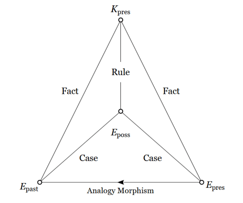

In logical terms, the analogy of experience proceeds by inducing a Rule about the validity of a current knowledge base and then by deducing a Fact, the applicability of that knowledge base to a current experience.
- Step 1 is Inductive, abstracting a Rule from a Case and a Fact.

- Step 2 is Deductive, admitting a Case to a Rule and arriving at a Fact.

References
- Awbrey, J.L., and Awbrey, S.M. (1995), “Interpretation as Action : The Risk of Inquiry”, Inquiry : Critical Thinking Across the Disciplines 15(1), 40–52. Archive. Journal. Online (doc) (pdf).
- Dewey, J. (1910), How We Think, D.C. Heath, Boston, MA. Reprinted (1991), Prometheus Books, Buffalo, NY. Online.
Resources
cc: Academia.edu • BlueSky • Laws of Form • Mathstodon • Research Gate
cc: Conceptual Graphs • Cybernetics • Structural Modeling • Systems Science


