I think the reader is beginning to get an inkling of the crucial importance of the “number of” function in Peirce’s way of looking at logic. It is one plank in the bridge from logic to the theories of probability, statistics, and information, in which setting logic forms but a limiting case at one scenic turnout on the expanding vista. It is one of the ways Peirce forges a link between the eternal, logical, or rational realm and the secular, empirical, or real domain.
With that note of encouragement and exhortation, let us return to the details of the text.
NOF 2
But not only do the significations of  and
and  here adopted fulfill all absolute requirements, but they have the supererogatory virtue of being very nearly the same as the common significations. Equality is, in fact, nothing but the identity of two numbers; numbers that are equal are those which are predicable of the same collections, just as terms that are identical are those which are predicable of the same classes. So, to write
  is to say that 5 is part of 7, just as to write
  is to say that Frenchmen are part of men. Indeed, if
  then the number of Frenchmen is less than the number of men, and if
  then the number of Vice‑Presidents is equal to the number of Presidents of the Senate; so that the numbers may always be substituted for the terms themselves, in case no signs of operation occur in the equations or inequalities.
(Peirce, CP 3.66)
Peirce observes that the measure  on logical terms preserves the relations of implication or inclusion which impose an ordering on those terms. Here Peirce uses a single symbol
  to denote the linear ordering on numbers, but also what amounts to the implication ordering on logical terms and the inclusion ordering on classes. Later he will introduce distinctive symbols for the logical orderings. The links among terms, sets, and numbers can be pursued in all directions and Peirce has already indicated in an earlier paper how he would construct the integers from sets, that is, from the aggregate denotations of terms. I will try to get back to that another time.
We have a statement of the following form.
If then the number of Frenchmen is less than the number of men.
This goes into symbolic form as follows.
![\begin{matrix} \mathrm{f} < \mathrm{m} & \Rightarrow & [\mathrm{f}] < [\mathrm{m}]. \end{matrix}](https://s0.wp.com/latex.php?latex=%5Cbegin%7Bmatrix%7D++%5Cmathrm%7Bf%7D+%3C+%5Cmathrm%7Bm%7D+%26+%5CRightarrow+%26+%5B%5Cmathrm%7Bf%7D%5D+%3C+%5B%5Cmathrm%7Bm%7D%5D.++%5Cend%7Bmatrix%7D&bg=ffffff&fg=000000&s=1&c=20201002)
In this setting the on the left is a logical ordering on syntactic terms while the on the right is an arithmetic ordering on real numbers.
The question that arises in this case is whether a map between two ordered sets is order-preserving. In order to formulate the question in more general terms, we may begin with the following set-up.
An order relation is typically defined by a set of axioms that determines its properties. Since we have frequent occasion to view the same set in the light of several different order relations, we often resort to explicit specifications like 
 and so on to indicate a set with a given ordering.
A map 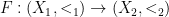 is order-preserving if and only if a statement of a particular form holds for all
  and
and  in
in  namely, the following.

The “number of” map  has just this character, as exemplified in the case at hand.
![\begin{matrix} \mathrm{f} & < & \mathrm{m} & \Rightarrow & [\mathrm{f}] & < & [\mathrm{m}] \\[6pt] \mathrm{f} & < & \mathrm{m} & \Rightarrow & v(\mathrm{f}) & < & v(\mathrm{m}) \end{matrix}](https://s0.wp.com/latex.php?latex=%5Cbegin%7Bmatrix%7D++%5Cmathrm%7Bf%7D+%26+%3C+%26+%5Cmathrm%7Bm%7D+%26+%5CRightarrow+%26+%5B%5Cmathrm%7Bf%7D%5D+%26+%3C+%26+%5B%5Cmathrm%7Bm%7D%5D++%5C%5C%5B6pt%5D++%5Cmathrm%7Bf%7D+%26+%3C+%26+%5Cmathrm%7Bm%7D+%26+%5CRightarrow+%26+v%28%5Cmathrm%7Bf%7D%29++%26+%3C+%26+v%28%5Cmathrm%7Bm%7D%29++%5Cend%7Bmatrix%7D&bg=ffffff&fg=000000&s=1&c=20201002)
The on the left is read as proper inclusion, in other words, subset of but not equal to, while the on the right is read as the usual less than relation.
Resources
cc: Cybernetics • Ontolog Forum • Structural Modeling • Systems Science
cc: FB | Peirce Matters • Laws of Form • Peirce List (1) (2) (3) (4) (5) (6) (7)


 is indicated by writing the term in square brackets, as
 ![[\mathit{t}].](https://s0.wp.com/latex.php?latex=%5B%5Cmathit%7Bt%7D%5D.&bg=ffffff&fg=000000&s=0&c=20201002) It is convenient to have a prefix notation for the function mapping a term
It is convenient to have a prefix notation for the function mapping a term ![[\mathit{t}]](https://s0.wp.com/latex.php?latex=%5B%5Cmathit%7Bt%7D%5D&bg=ffffff&fg=000000&s=0&c=20201002) but Peirce previously reserved the letter
but Peirce previously reserved the letter  for logical
  so let’s use
  as a variant for
  The number of a relative with two correlates would be the average number of things so related to a pair of individuals; and so on for relatives of higher numbers of correlates. I propose to denote the number of a logical term by enclosing the term in square brackets, thus
  where
where  is a suitable set of signs, a syntactic domain, containing all the logical terms whose numbers we need to evaluate in a given context, and where
  is the set of real numbers.
 ![\begin{array}{ll} \text{Let} & \mathrm{m} ~=~ \text{man} \\[8pt] \text{and} & \mathit{t} ~=~ \text{tooth of}\,\underline{~~~~}. \\[8pt] \text{Then} & v(\mathit{t}) ~=~ [\mathit{t}] ~=~ \displaystyle\frac{[\mathit{t}\mathrm{m}]}{[\mathrm{m}]}. \end{array}](https://s0.wp.com/latex.php?latex=%5Cbegin%7Barray%7D%7Bll%7D++%5Ctext%7BLet%7D++%26+%5Cmathrm%7Bm%7D+%7E%3D%7E+%5Ctext%7Bman%7D++%5C%5C%5B8pt%5D++%5Ctext%7Band%7D++%26+%5Cmathit%7Bt%7D+%7E%3D%7E+%5Ctext%7Btooth+of%7D%5C%2C%5Cunderline%7B%7E%7E%7E%7E%7D.++%5C%5C%5B8pt%5D++%5Ctext%7BThen%7D+%26+v%28%5Cmathit%7Bt%7D%29+%7E%3D%7E+%5B%5Cmathit%7Bt%7D%5D+%7E%3D%7E+%5Cdisplaystyle%5Cfrac%7B%5B%5Cmathit%7Bt%7D%5Cmathrm%7Bm%7D%5D%7D%7B%5B%5Cmathrm%7Bm%7D%5D%7D.++%5Cend%7Barray%7D&bg=ffffff&fg=000000&s=1&c=20201002)
 in a universe of perfect human dentition is equal to the number of teeth of humans divided by the number of humans, that is,
  where
where  and
and  contain all the teeth and all the people, respectively, under discussion.
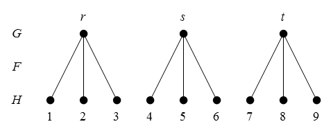
 might be drawn as follows, showing just the first few items in the toothy part of

 needs the data represented by the entire bigraph for
  since we are counting only teeth which occupy exactly one mouth of a tooth-bearing creature.
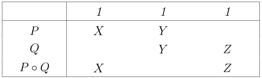
 we have the following data.
![\begin{array}{lcccll} J & : & \mathbb{R} & \gets & \mathbb{R} & \text{(properly restricted)} \\[6pt] K & : & \mathbb{R} & \gets & \mathbb{R} \times \mathbb{R} & \text{where}~ K(r, s) = r + s \\[6pt] L & : & \mathbb{R} & \gets & \mathbb{R} \times \mathbb{R} & \text{where}~ L(u, v) = u \cdot v \end{array}](https://s0.wp.com/latex.php?latex=%5Cbegin%7Barray%7D%7Blcccll%7D++J+%26+%3A+%26+%5Cmathbb%7BR%7D+%26+%5Cgets+%26+%5Cmathbb%7BR%7D+%26+%5Ctext%7B%28properly+restricted%29%7D++%5C%5C%5B6pt%5D++K+%26+%3A+%26+%5Cmathbb%7BR%7D+%26+%5Cgets+%26+%5Cmathbb%7BR%7D+%5Ctimes+%5Cmathbb%7BR%7D+%26+%5Ctext%7Bwhere%7D%7E+K%28r%2C+s%29+%3D+r+%2B+s++%5C%5C%5B6pt%5D++L+%26+%3A+%26+%5Cmathbb%7BR%7D+%26+%5Cgets+%26+%5Cmathbb%7BR%7D+%5Ctimes+%5Cmathbb%7BR%7D+%26+%5Ctext%7Bwhere%7D%7E+L%28u%2C+v%29+%3D+u+%5Ccdot+v++%5Cend%7Barray%7D&bg=ffffff&fg=000000&s=1&c=20201002)
![\begin{matrix} J & : & [+] \gets [\,\cdot\,] \\[6pt] [+] & \subseteq & \mathbb{R} \times \mathbb{R} \times \mathbb{R} \\[6pt] [\,\cdot\,] & \subseteq & \mathbb{R} \times \mathbb{R} \times \mathbb{R} \end{matrix}](https://s0.wp.com/latex.php?latex=%5Cbegin%7Bmatrix%7D++J+%26+%3A+%26+%5B%2B%5D+%5Cgets+%5B%5C%2C%5Ccdot%5C%2C%5D++%5C%5C%5B6pt%5D++%5B%2B%5D+%26+%5Csubseteq+%26+%5Cmathbb%7BR%7D+%5Ctimes+%5Cmathbb%7BR%7D+%5Ctimes+%5Cmathbb%7BR%7D++%5C%5C%5B6pt%5D++%5B%5C%2C%5Ccdot%5C%2C%5D+%26+%5Csubseteq+%26+%5Cmathbb%7BR%7D+%5Ctimes+%5Cmathbb%7BR%7D+%5Ctimes+%5Cmathbb%7BR%7D++%5Cend%7Bmatrix%7D&bg=ffffff&fg=000000&s=1&c=20201002)
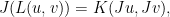
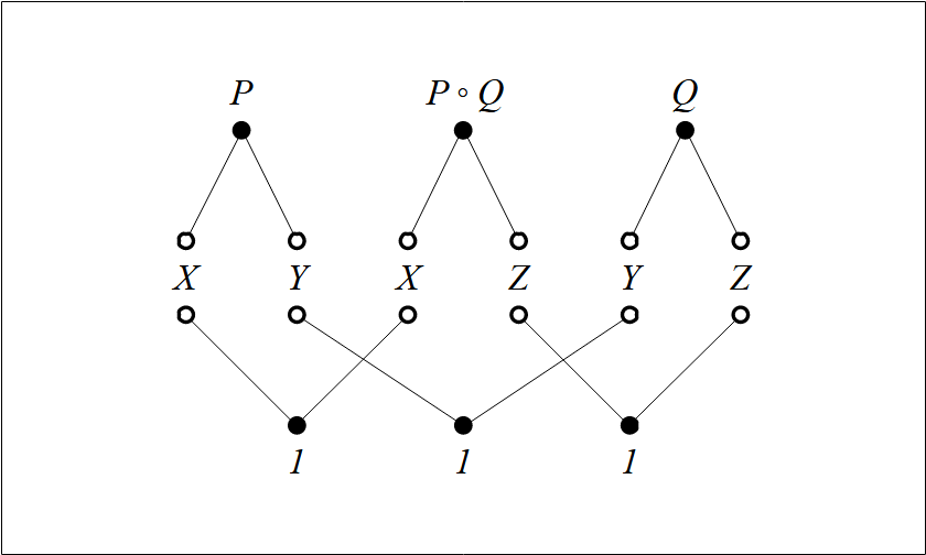
 or simple concatenation, but they remain in general distinct whether considered as operations or as relations, no matter what signs of operation are used. In such a setting, our chiasmatic theme may run a bit like one of the following two variants.

 and
and 

 takes on the shape
  which looks analogous to the distributive multiplication of a factor
  That is why morphisms are regarded as generalizations of linear functions and are frequently referred to in those terms.
 say, one of the mappings of reals into reals commonly known as logarithm functions, where you get to pick your favorite base.
 and
and  and the formula
  becomes
 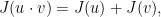 where ordinary multiplication and addition are indicated by a dot
  and a plus sign
  respectively.

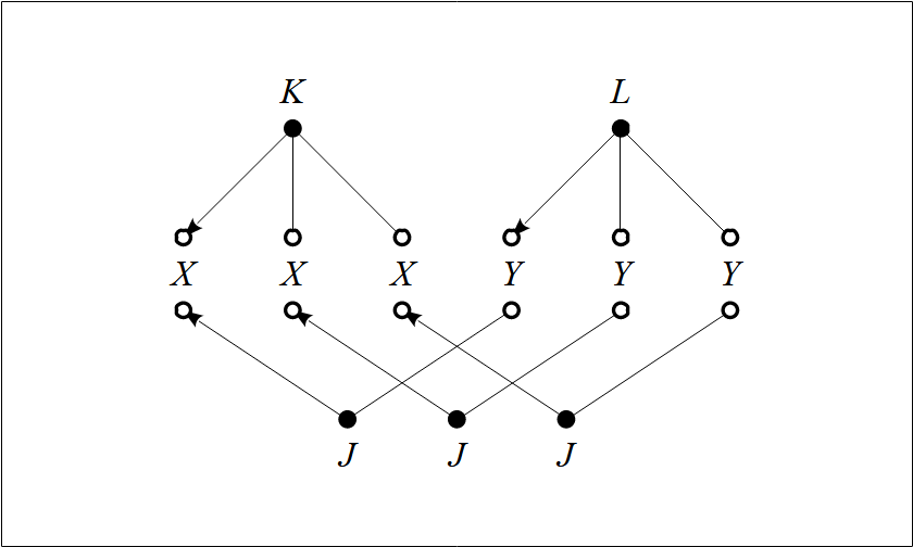
 satisfying the following conditions.
![\begin{array}{lcccl} J & : & X & \gets & Y \\[6pt] K & : & X & \gets & X \times X \\[6pt] L & : & Y & \gets & Y \times Y \end{array}](https://s0.wp.com/latex.php?latex=%5Cbegin%7Barray%7D%7Blcccl%7D++J+%26+%3A+%26+X+%26+%5Cgets+%26+Y++%5C%5C%5B6pt%5D++K+%26+%3A+%26+X+%26+%5Cgets+%26+X+%5Ctimes+X++%5C%5C%5B6pt%5D++L+%26+%3A+%26+Y+%26+%5Cgets+%26+Y+%5Ctimes+Y++%5Cend%7Barray%7D&bg=ffffff&fg=000000&s=1&c=20201002)


 row along with all the constraints in the
  row. Quite by design, that is one way to understand the equation

 and
and  are assumed to be functional on correlates, a premiss we express as follows.
 is also functional on correlates, in symbols, whether
 we have the following equivalence.
 For that we have the following formula, where the summation indicated is logical disjunction.
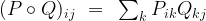
 or the fact that
  means there is exactly one ordered pair
  for each
 or the fact that
  means there is exactly one ordered pair
  for each
 for each
  which means
  and so we have the function
  and the corresponding relation
  are both called functional on rèlates if and only if
  We write this in symbols as


 and
and 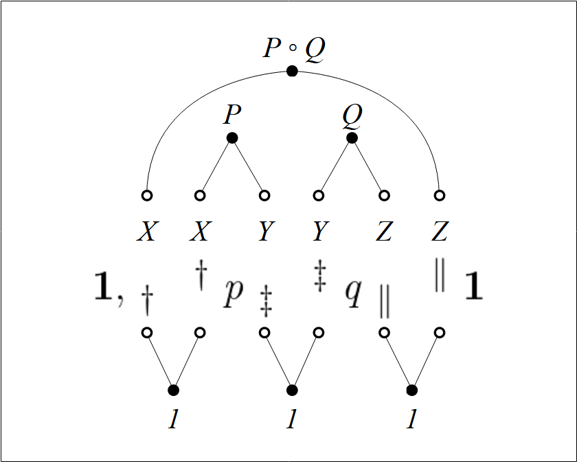


 which qualifies as a function
  may then enjoy a number of further distinctions.
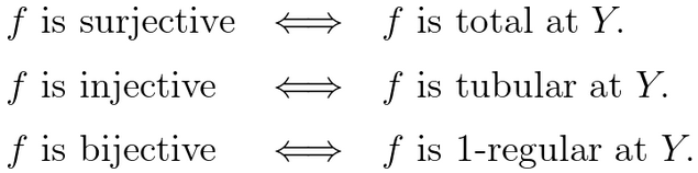

 above is
 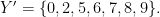 If we form a new function
  that looks just like
  then
then  is surjective, and is described as a mapping onto

 is injective.
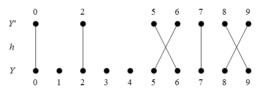

 is bijective.

 -regularity conditions where
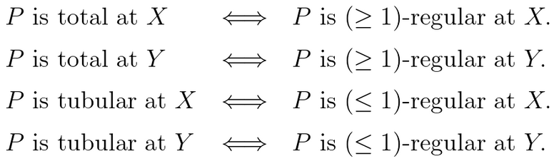
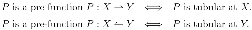
 -regular, total and tubular, or total prefunctions on specified domains,
  that happens to be total at
  then
then  typically indicated as
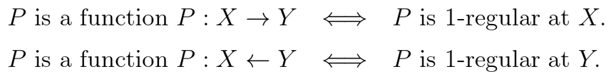
 and let
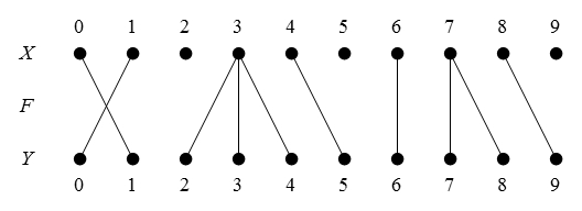

 is a function at
  or
or 
 if and only if the cardinality of the local flag
  is equal to
  coded in symbols, if and only if
  for all
 and so on. For ease of reference, a number of such definitions are recorded below.
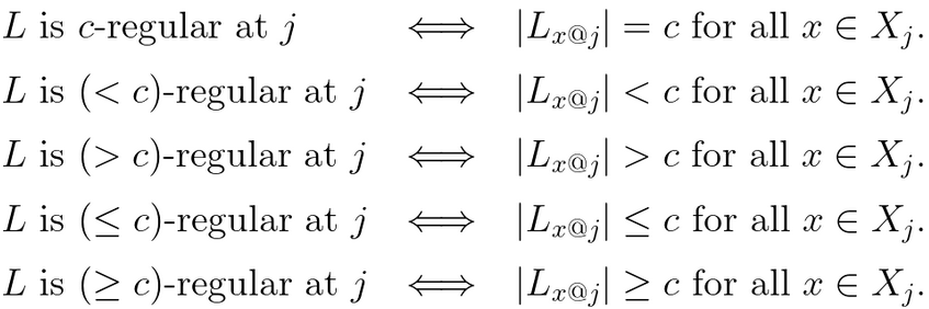
 on one of its domains
  and also
  on the same domain, then it must be
  on that domain, in short,
  at
at 
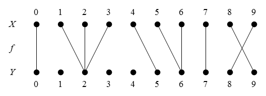
 and
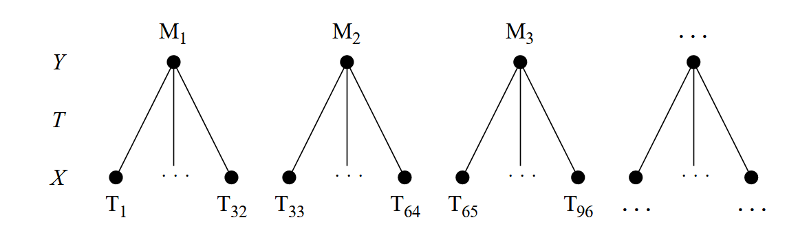
and  and consider the dyadic relation
  bigraphed below.