
Peirce’s 1870 “Logic of Relatives” • Comment 11.13
As we make our way toward the foothills of Peirce’s 1870 Logic of Relatives there are several pieces of equipment we must not leave the plains without, namely, the utilities variously known as arrows, morphisms, homomorphisms, structure-preserving maps, among other names, depending on the altitude of abstraction we happen to be traversing at the moment in question. As a moderate to middling but not too beaten track, let’s examine a few ways of defining morphisms that will serve us in the present discussion.
Suppose we are given three functions 
![\begin{array}{lcccl} J & : & X & \gets & Y \\[6pt] K & : & X & \gets & X \times X \\[6pt] L & : & Y & \gets & Y \times Y \end{array}](https://s0.wp.com/latex.php?latex=%5Cbegin%7Barray%7D%7Blcccl%7D++J+%26+%3A+%26+X+%26+%5Cgets+%26+Y++%5C%5C%5B6pt%5D++K+%26+%3A+%26+X+%26+%5Cgets+%26+X+%5Ctimes+X++%5C%5C%5B6pt%5D++L+%26+%3A+%26+Y+%26+%5Cgets+%26+Y+%5Ctimes+Y++%5Cend%7Barray%7D&bg=ffffff&fg=000000&s=1&c=20201002)

Our sagittarian leitmotif can be rubricized in the following slogan.
The J-image of the L-product is the K-product of the J-images.
Figure 47 presents us with a picture of the situation in question.
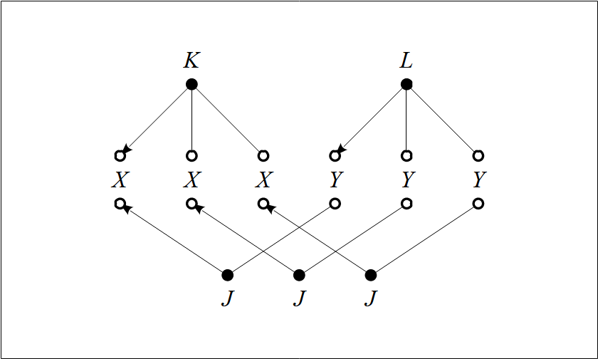

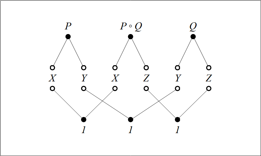
Table 48 gives the constraint matrix version of the same thing.

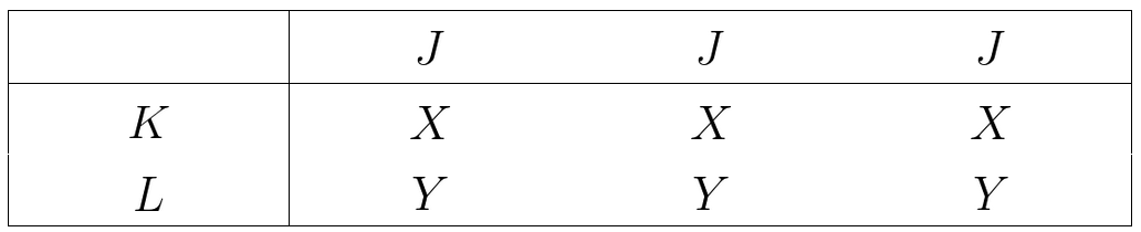
One way to read the Table is in terms of the informational redundancies it summarizes. For example, one way to read it says that satisfying the constraint in the 


Resources
- Peirce’s 1870 Logic of Relatives • Part 1 • Part 2 • Part 3 • References
- Logic Syllabus • Relational Concepts • Relation Theory • Relative Term
cc: Cybernetics • Ontolog Forum • Structural Modeling • Systems Science
cc: FB | Peirce Matters • Laws of Form • Peirce List (1) (2) (3) (4) (5) (6) (7)

 and
and  are assumed to be functional on correlates, a premiss we express as follows.
 is also functional on correlates, in symbols, whether
 we have the following equivalence.
 For that we have the following formula, where the summation indicated is logical disjunction.
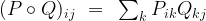
 or the fact that
 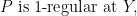 means there is exactly one ordered pair
  for each
 or the fact that
  means there is exactly one ordered pair
  for each
 for each
  which means
  and so we have the function
  and the corresponding relation
  are both called functional on rèlates if and only if
  We write this in symbols as
 We write this in symbols as

 and
and 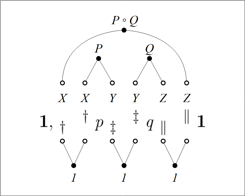


 which qualifies as a function
  may then enjoy a number of further distinctions.
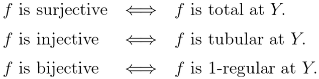
 so it can enjoy none of the properties of being surjective, injective, or bijective.
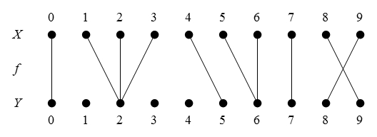

 above is
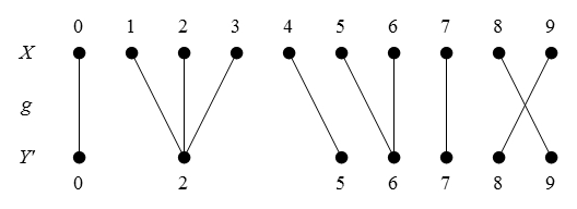
 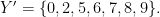 If we form a new function
  that looks just like
  but is assigned the codomain
  then
then  is surjective, and is described as a mapping onto

 is injective.
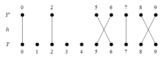

 is bijective.

 -regularity conditions where
 -regular, total and tubular, or total prefunctions on specified domains,
  that happens to be total at
  then
then  typically indicated as
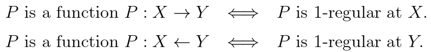
 and let
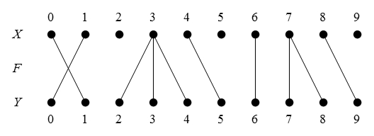

 is a function at
  or
or 
 if and only if the cardinality of the local flag
  is equal to
  in
in  coded in symbols, if and only if
  for all
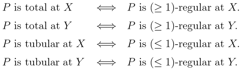
 and so on. For ease of reference, a number of such definitions are recorded below.
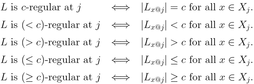
 on one of its domains
  and also
  on the same domain, then it must be
  on that domain, in short,
  at
at 
 and
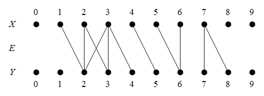
and  and consider the dyadic relation
  bigraphed below.
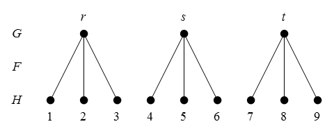

 and 1-regular at
 of a
of a  -adic relation

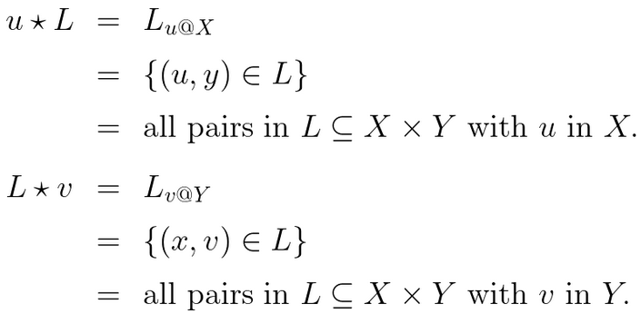
 the notation for local flags can be simplified in two ways. First, the local flags
  and
and  are often more conveniently notated as
  and
and  respectively. Second, the notation may be streamlined even further by making the following definitions.
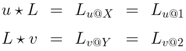


 of
of 

 of
of 

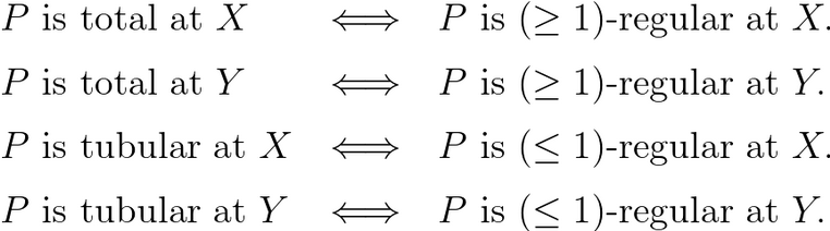
 exemplifies the quality of totality at
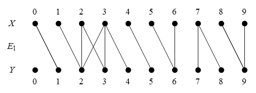
 exemplifies the quality of totality at

 exemplifies the quality of tubularity at

 exemplifies the quality of tubularity at
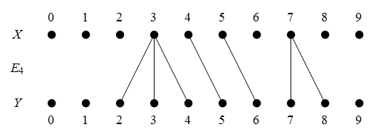
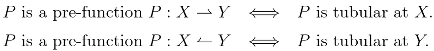
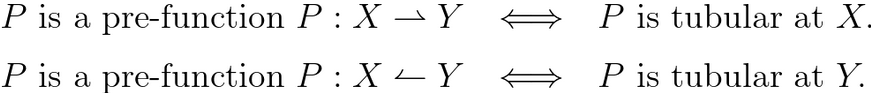
 is a pre-function
  and
and  is a pre-function
 and writing
 where
where  and where the bigraph picture of
  is shown in Figure 30.
 to
to  we see that the incidence degrees of the
  in that order.
 in that order.
 in the following way.
![v(t) ~:=~ [t] ~=~ \text{the number of the term}~ t.](https://s0.wp.com/latex.php?latex=v%28t%29+%7E%3A%3D%7E+%5Bt%5D+%7E%3D%7E+%5Ctext%7Bthe+number+of+the+term%7D%7E+t.&bg=ffffff&fg=000000&s=1&c=20201002)
 where
where  is the set of real numbers and
  is a suitable syntactic domain, here described as a set of terms. The dyadic relation
  is at first sight a function from
  It is, however, not always possible to assign a number to every term in whatever syntactic domain
  means
means  is functional at
 means
means 
 means
means  means
means  written
  amounting to a functional alias of the dyadic relation