
Transfer
What exactly gives the acquisition of a knowledge base its distinctively inductive character? It is evidently the “analogy of experience” involved in applying what we’ve learned in the past to what confronts us in the present.
Whenever we find ourselves approaching a problem with the thought, If past experience is any guide … we can be sure the analogy of experience has come into play. We are seeking to find analogies between past experience as a totality and present experience as a point of application.
From a statistical point of view what we mean is this — “If past experience is a fair sample of possible experience then knowledge gained from past experience may usefully apply to present experience”. It is that mechanism which allows a knowledge base to be carried across gulfs of experience which remain indifferent to the effective contents of its rules.
Next we’ll examine how the transfer of knowledge through the analogy of experience works out in the case of Dewey’s “Sign of Rain” example.
References
- Awbrey, J.L., and Awbrey, S.M. (1995), “Interpretation as Action : The Risk of Inquiry”, Inquiry : Critical Thinking Across the Disciplines 15(1), 40–52. Archive. Journal. Online (doc) (pdf).
- Dewey, J. (1910), How We Think, D.C. Heath, Boston, MA. Reprinted (1991), Prometheus Books, Buffalo, NY. Online.
Resources
- Survey of Abduction, Deduction, Induction, Analogy, Inquiry
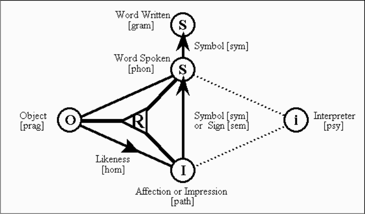
- Survey of Semiotics, Semiosis, Sign Relations
cc: Academia.edu • BlueSky • Laws of Form • Mathstodon • Research Gate
cc: Conceptual Graphs • Cybernetics • Structural Modeling • Systems Science


 In the Current situation the Air is cool.
 Just Before it rains, the Air is cool.
 The Current situation is just Before it rains.
 Just Before it rains, a Dark cloud will appear.
 In the Current situation, a Dark cloud will appear.


 are shown in the next two Figures.

![[\mathcal{X}] \to [\mathcal{Y}]](https://s0.wp.com/latex.php?latex=%5B%5Cmathcal%7BX%7D%5D+%5Cto+%5B%5Cmathcal%7BY%7D%5D&bg=ffffff&fg=000000&s=0&c=20201002) is implied any time we make use of one basis
is implied any time we make use of one basis  which happens to be included in another basis
  When discussing differential relations we usually have in mind the extended alphabet
  has a special construction or a specific lexical relation with respect to the initial alphabet
  one which is marked by characteristic types of accents, indices, or inflected forms.