A differential propositional calculus is a propositional calculus extended by a set of terms for describing aspects of change and difference, for example, processes taking place in a universe of discourse or transformations mapping a source universe to a target universe.
Casual Introduction
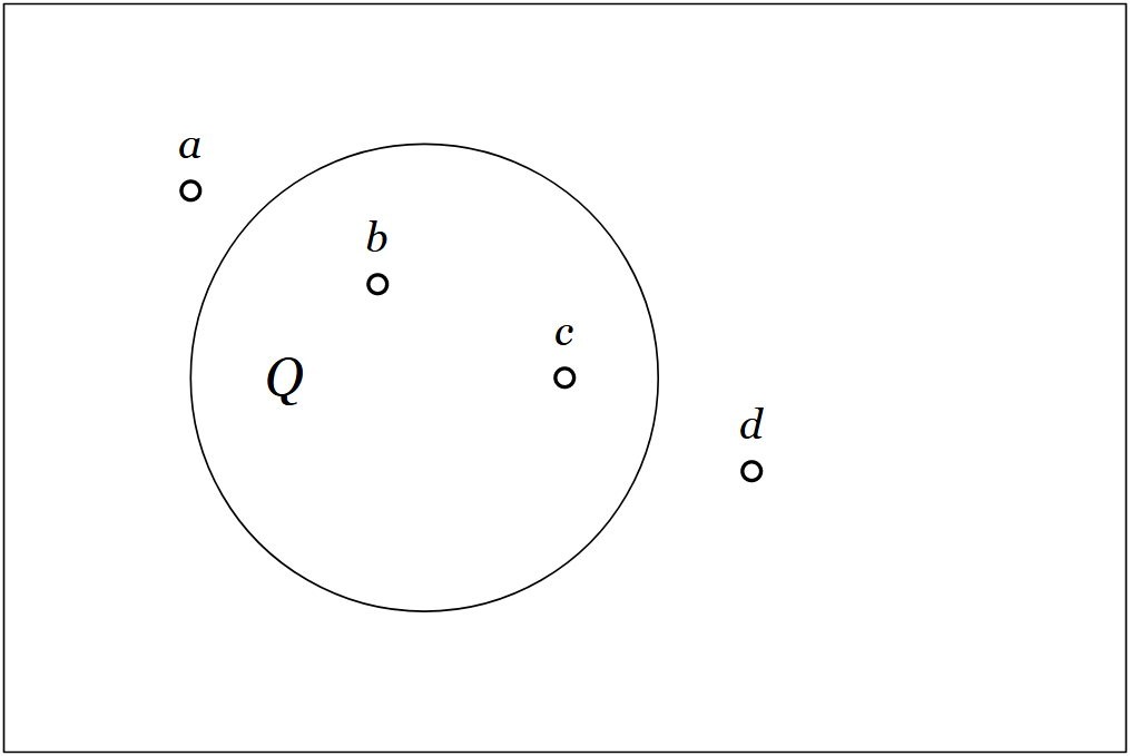
Consider the situation represented by the venn diagram in Figure 1.

The area of the rectangle represents a universe of discourse,  The universe under discussion may be a population of individuals having various additional properties or it may be a collection of locations occupied by various individuals. The area of the “circle” represents the individuals having the property
  or the locations in the corresponding region
  Four individuals,
  are singled out by name. It happens that
  and
and  currently reside in region
  while
while  and
and  do not.
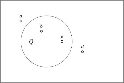
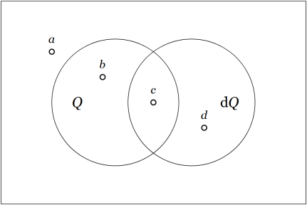
Now consider the situation represented by the venn diagram in Figure 2.
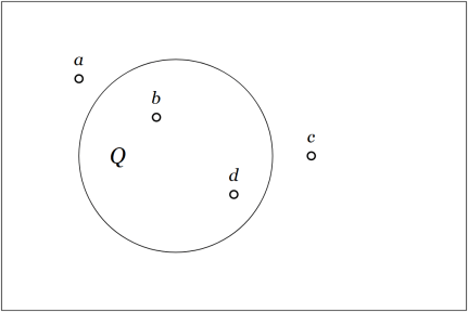

Figure 2 differs from Figure 1 solely in the circumstance that the object is outside the region while the object is inside the region So far, nothing says our encountering these Figures in this order is other than purely accidental but if we interpret this sequence of frames as a “moving picture” representation of their natural order in a temporal process then it would be natural to suppose and have remained as they were with regard to the quality while and have changed their standings in that respect. In particular, has moved from the region where is true to the region where is false while has moved from the region where is false to the region where is true.
Figure 3 returns to the situation in Figure 1, but this time interpolates a new quality specifically tailored to account for the relation between Figure 1 and Figure 2.

This new quality,  is an example of a differential quality, since its absence or presence qualifies the absence or presence of change occurring in another quality. As with any other quality, it is represented in the venn diagram by means of a “circle” distinguishing two halves of the universe of discourse, in this case, the portions of
  outside and inside the region
Figure 1 represents a universe of discourse,  together with a basis of discussion,
  for expressing propositions about the contents of that universe. Once the quality is given a name, say, the symbol
  we have the basis for a formal language specifically cut out for discussing in terms of
  This language is more formally known as the propositional calculus with alphabet
In the context marked by and  there are just four distinct pieces of information which can be expressed in the corresponding propositional calculus, namely, the constant proposition
  the negative proposition
  the positive proposition
  and the constant proposition
For example, referring to the points in Figure 1, the constant proposition  holds of no points, the negative proposition
  holds of and
  the positive proposition holds of and
  and the constant proposition
  holds of all points in the sample.
Figure 3 extends the basis of description for the space to a set of two qualities  and the corresponding terms of description to an alphabet of two symbols
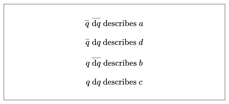
Any propositional calculus over two basic propositions allows for the expression of sixteen propositions all together. Salient among those propositions in the present setting are the four which single out the individual sample points at the initial moment of observation. Table 4 lists the initial state descriptions, using overlines to express logical negations.


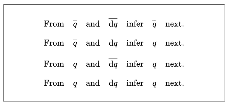
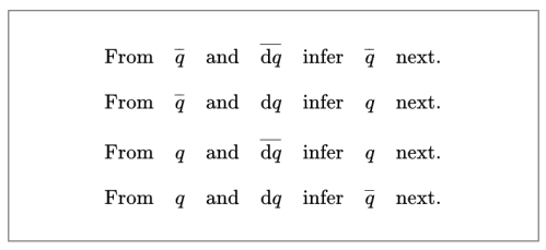
Table 5 shows the rules of inference responsible for giving the differential quality  its meaning in practice.

Resources
cc: Cybernetics • Ontolog Forum • Peirce List • Structural Modeling • Systems Science


is extended by a first order differential alphabet
resulting in a first order extended alphabet
defined as follows.
is extended by a first order differential basis
resulting in a first order extended basis
defined as follows.
is extended by a first order differential space or tangent space
at each point of
resulting in a first order extended space or tangent bundle space
defined as follows.
is extended by a first order differential universe or tangent universe
at each point of
resulting in a first order extended universe or tangent bundle universe


![\mathrm{E}A^\bullet ~=~ [ \mathrm{E}\mathcal{A} ] ~=~ [ \mathcal{A} ~\cup~ \mathrm{d}\mathcal{A} ] ~=~ [ a_1, \ldots, a_n, \mathrm{d}a_1, \ldots, \mathrm{d}a_n ].](https://s0.wp.com/latex.php?latex=%5Cmathrm%7BE%7DA%5E%5Cbullet+%7E%3D%7E+%5B+%5Cmathrm%7BE%7D%5Cmathcal%7BA%7D+%5D+%7E%3D%7E+%5B+%5Cmathcal%7BA%7D+%7E%5Ccup%7E+%5Cmathrm%7Bd%7D%5Cmathcal%7BA%7D+%5D+%7E%3D%7E+%5B+a_1%2C+%5Cldots%2C+a_n%2C+%5Cmathrm%7Bd%7Da_1%2C+%5Cldots%2C+%5Cmathrm%7Bd%7Da_n+%5D.&bg=ffffff&fg=000000&s=0&c=20201002)
![[ \mathbb{B}^n \times \mathbb{D}^n ] ~=~ (\mathbb{B}^n \times \mathbb{D}^n\ +\!\!\to \mathbb{B}) ~=~ (\mathbb{B}^n \times \mathbb{D}^n, \mathbb{B}^n \times \mathbb{D}^n \to \mathbb{B}).](https://s0.wp.com/latex.php?latex=%5B+%5Cmathbb%7BB%7D%5En+%5Ctimes+%5Cmathbb%7BD%7D%5En+%5D+%7E%3D%7E+%28%5Cmathbb%7BB%7D%5En+%5Ctimes+%5Cmathbb%7BD%7D%5En%5C+%2B%5C%21%5C%21%5Cto+%5Cmathbb%7BB%7D%29+%7E%3D%7E+%28%5Cmathbb%7BB%7D%5En+%5Ctimes+%5Cmathbb%7BD%7D%5En%2C+%5Cmathbb%7BB%7D%5En+%5Ctimes+%5Cmathbb%7BD%7D%5En+%5Cto+%5Cmathbb%7BB%7D%29.&bg=ffffff&fg=000000&s=0&c=20201002)


 singular propositions are those singling out the minimal distinct regions of the universe, represented by single cells of the corresponding venn diagram.
 there are
  singular propositions. Their venn diagrams are shown in Figure 10.
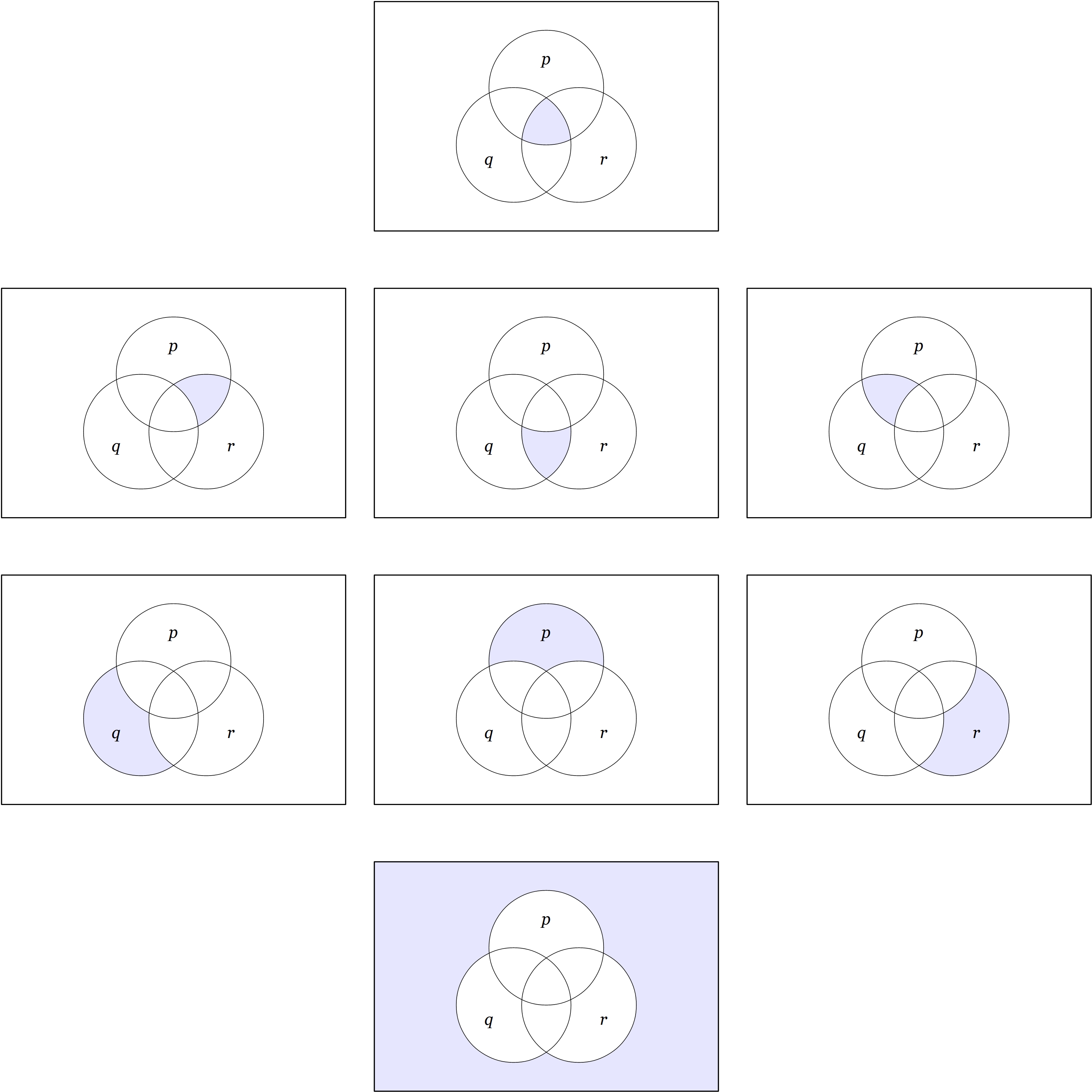

 and identical with the positive proposition of rank 3.


 respectively.
 function, which may be expressed by the form
  or by a simple

 are added “modulo 2”, that is, in such a way that


 function, which may be expressed by the form
  or by a simple
![A^\bullet = [a_1, \ldots, a_n]](https://s0.wp.com/latex.php?latex=A%5E%5Cbullet+%3D+%5Ba_1%2C+%5Cldots%2C+a_n%5D&bg=ffffff&fg=000000&s=0&c=20201002) qualified by the logical features
qualified by the logical features  is a set
  plus the set of all functions from the space
  There are
  elements in
  possible functions from
  accordingly pictured as all the ways of painting the cells of a venn diagram or the nodes of a hypercube with a palette of two colors.
 evaluates to
  The analogy between logical propositions and boolean-valued functions is close enough to adopt the latter as models of the former and simply refer to the functions
 ![[a_1, \ldots, a_n]](https://s0.wp.com/latex.php?latex=%5Ba_1%2C+%5Cldots%2C+a_n%5D&bg=ffffff&fg=000000&s=0&c=20201002) is one of the propositions in the set
is one of the propositions in the set  There are of course exactly
  of these. Depending on the context, basic propositions may also be called coordinate propositions or simple propositions.
 and falls into
  ranks, with a binomial coefficient
  giving the number of propositions having rank or weight
  in their class.
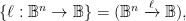 may be written as sums:
 may be written as products:
 may be written as products:
 the linear proposition of rank
  the positive proposition of rank
  and the singular proposition of rank
 are both linear and positive. So these two kinds of propositions, the linear and the positive, may be viewed as two different ways of generalizing the class of basic propositions.
 A singular proposition with respect to the basis
  will not remain singular if
  to pick out a new basis, the sets of linear propositions and positive propositions are both determined by the choice of basic propositions, and this whole determination is tantamount to the purely conventional choice of a cell as origin.
 The signs are interpreted as denoting logical features, for example, properties of objects in the universe of discourse or simple propositions about those objects. Corresponding to the alphabet
  there is then a set of logical features,
 ![A^\bullet = [ \mathcal{A} ] = [ a_1, \ldots, a_n ].](https://s0.wp.com/latex.php?latex=A%5E%5Cbullet+%3D+%5B+%5Cmathcal%7BA%7D+%5D+%3D+%5B+a_1%2C+%5Cldots%2C+a_n+%5D.&bg=ffffff&fg=000000&s=0&c=20201002) It is useful to consider a universe of discourse as a categorical object incorporating both the set of points
It is useful to consider a universe of discourse as a categorical object incorporating both the set of points  implicit with the ordinary picture of a venn diagram on
  having the type
  and this last type designation may be abbreviated as
  or even more succinctly as
 ![[ \mathbb{B}^n ].](https://s0.wp.com/latex.php?latex=%5B+%5Cmathbb%7BB%7D%5En+%5D.&bg=ffffff&fg=000000&s=0&c=20201002) For convenience, the data type of a finite set on
For convenience, the data type of a finite set on ![[n]](https://s0.wp.com/latex.php?latex=%5Bn%5D&bg=ffffff&fg=000000&s=0&c=20201002) or
or 


 is taken to mean exactly one of the propositions
  is false, in other words, their
  is taken to mean every one of the propositions

 or barred parentheses
  may be used for logical operators.
 or
or  in formal languages, where it forms the identity element for concatenation. It may be given visible expression in this context by means of the logically equivalent form
  or, especially if operating in an algebraic context, by a simple
  may be used for
 ![\begin{matrix} x + y ~=~ \texttt{(} x \texttt{,} y \texttt{)} \\[6pt] x + y + z ~=~ \texttt{((} x \texttt{,} y \texttt{),} z \texttt{)} ~=~ \texttt{(} x \texttt{,(} y \texttt{,} z \texttt{))} \end{matrix}](https://s0.wp.com/latex.php?latex=%5Cbegin%7Bmatrix%7D++x+%2B+y+%7E%3D%7E+%5Ctexttt%7B%28%7D+x+%5Ctexttt%7B%2C%7D+y+%5Ctexttt%7B%29%7D++%5C%5C%5B6pt%5D++x+%2B+y+%2B+z+%7E%3D%7E+%5Ctexttt%7B%28%28%7D+x+%5Ctexttt%7B%2C%7D+y+%5Ctexttt%7B%29%2C%7D+z+%5Ctexttt%7B%29%7D+%7E%3D%7E+%5Ctexttt%7B%28%7D+x+%5Ctexttt%7B%2C%28%7D+y+%5Ctexttt%7B%2C%7D+z+%5Ctexttt%7B%29%29%7D++%5Cend%7Bmatrix%7D&bg=ffffff&fg=000000&s=0&c=20201002)