Special Classes of Propositions (concl.)
Last and literally least in extent, we examine the family of singular propositions in a 3‑dimensional universe of discourse.
In our model of propositions as mappings from a universe of discourse  to a set of two values, in other words, indicator functions of the form
  singular propositions are those singling out the minimal distinct regions of the universe, represented by single cells of the corresponding venn diagram.
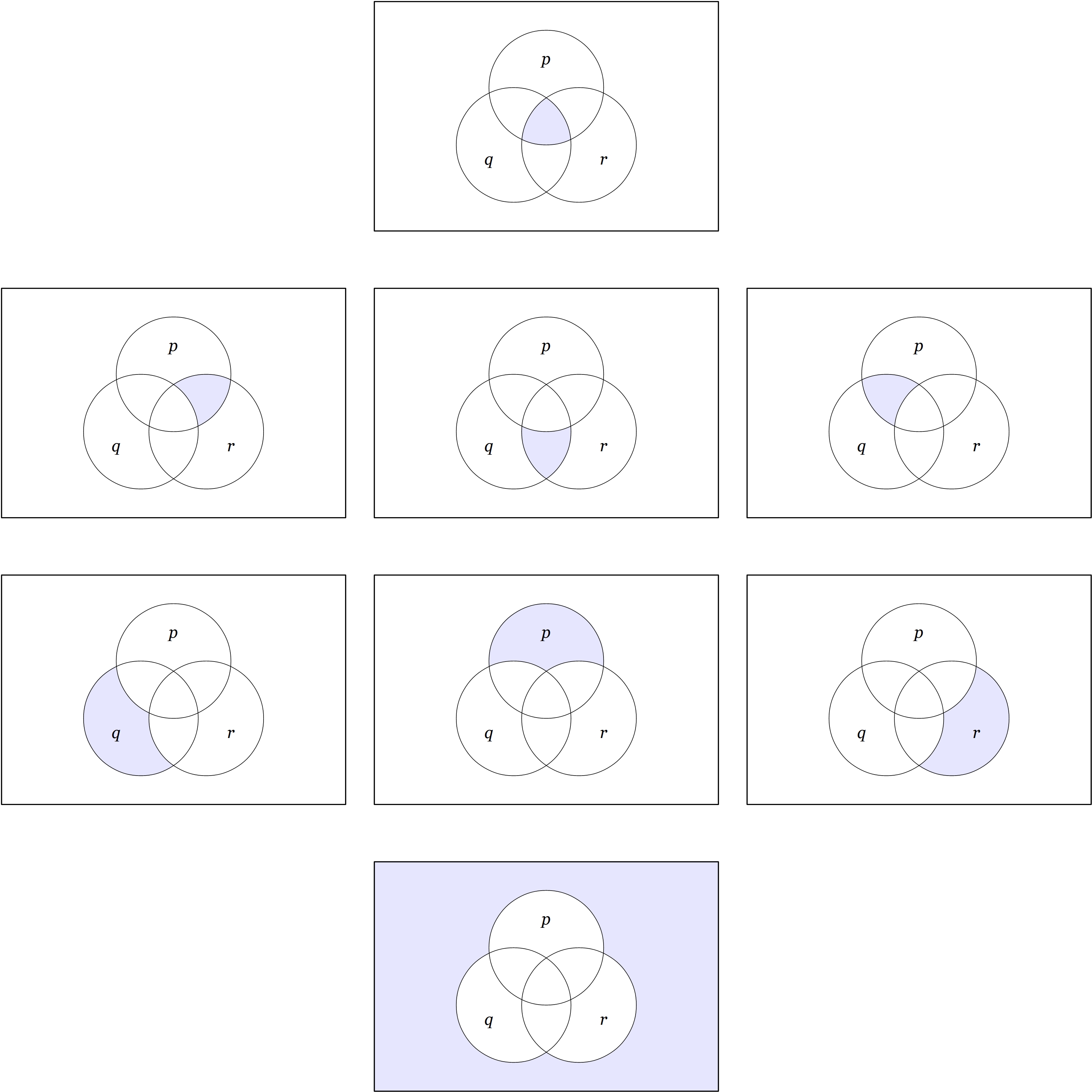
Singular Propositions
The singular propositions,  may be written as products:

In a universe of discourse based on three boolean variables,  there are
  singular propositions. Their venn diagrams are shown in Figure 10.


At the top is the venn diagram for the singular proposition of rank 3, corresponding to the boolean product  and identical with the positive proposition of rank 3.
Next are the venn diagrams for the three singular propositions of rank 2, which may be expressed by the following three forms, respectively.

Next are the three singular propositions of rank 1, which may be expressed by the following three forms, respectively.

At the bottom is the singular proposition of rank 0, which may be expressed by the following form.

Resources
cc: Academia.edu • Cybernetics • Structural Modeling • Systems Science
cc: Conceptual Graphs • Laws of Form • Mathstodon • Research Gate


![\mathcal{X}^\bullet = [\mathcal{X}],](https://s0.wp.com/latex.php?latex=%5Cmathcal%7BX%7D%5E%5Cbullet+%3D+%5B%5Cmathcal%7BX%7D%5D%2C&bg=ffffff&fg=000000&s=0&c=20201002)

![[\mathrm{E}\mathcal{A}]](https://s0.wp.com/latex.php?latex=%5B%5Cmathrm%7BE%7D%5Cmathcal%7BA%7D%5D&bg=ffffff&fg=000000&s=0&c=20201002) makes the task of solving differential propositions relatively straightforward. The solution set of the differential proposition
makes the task of solving differential propositions relatively straightforward. The solution set of the differential proposition  is the set of models
  in
in  Finding all models of
  the extended interpretations in
  which satisfy
  of a universe of discourse
 ![[\mathcal{A}]](https://s0.wp.com/latex.php?latex=%5B%5Cmathcal%7BA%7D%5D&bg=ffffff&fg=000000&s=0&c=20201002) is formed by taking the initial basis
is formed by taking the initial basis  together with the differential basis
  Thus we have the following formula.
 also called the tangent bundle of


![\mathrm{E}A^\bullet = [\mathrm{E}\mathcal{A}]](https://s0.wp.com/latex.php?latex=%5Cmathrm%7BE%7DA%5E%5Cbullet+%3D+%5B%5Cmathrm%7BE%7D%5Cmathcal%7BA%7D%5D&bg=ffffff&fg=000000&s=0&c=20201002) is the full collection of points and functions, or interpretations and propositions, based on the extended set of features
is the full collection of points and functions, or interpretations and propositions, based on the extended set of features  a fact summed up in the following notation.
![\mathrm{E}A^\bullet ~=~ [\mathrm{E}\mathcal{A}] ~=~ [a_1, \ldots, a_n, \mathrm{d}a_1, \ldots, \mathrm{d}a_n]](https://s0.wp.com/latex.php?latex=%5Cmathrm%7BE%7DA%5E%5Cbullet+%7E%3D%7E+%5B%5Cmathrm%7BE%7D%5Cmathcal%7BA%7D%5D+%7E%3D%7E+%5Ba_1%2C+%5Cldots%2C+a_n%2C+%5Cmathrm%7Bd%7Da_1%2C+%5Cldots%2C+%5Cmathrm%7Bd%7Da_n%5D&bg=ffffff&fg=000000&s=0&c=20201002)
 the following type.
 we arrive at the launchpad of our space explorations.

 taken by itself. In like fashion, the adjective extended or the substantive bundle is systematically attached to any construct associated with the full complement of
  features.
 sometimes written
  takes the form


 Strictly speaking, the name cotangent space is probably more correct for this construction but since we take up spaces and their duals in pairs to form our universes of discourse it allows our language to be pliable here.
 is a set consisting of two differential propositions,
  where
where  is a proposition with the logical value of
  Each component
  operating under the ordered correspondence
  A measure of clarity is achieved, however, by acknowledging the differential usage with a superficially distinct type
  whose sense may be indicated as follows.
 and
and  may appear to be identical sets of binary vectors, but taking a view at that level of abstraction would be like ignoring the qualitative units and the diverse dimensions that distinguish position and momentum, or the different roles of quantity and impulse.
 with a set of symbols for differential features, in effect basic changes capable of occurring in
 ![[\mathcal{A}].](https://s0.wp.com/latex.php?latex=%5B%5Cmathcal%7BA%7D%5D.&bg=ffffff&fg=000000&s=0&c=20201002) The additional symbols are taken to denote primitive features of change, qualitative attributes of motion, or proposals about the ways items in the universe of discourse may change or move in relation to features noted in the original alphabet.
The additional symbols are taken to denote primitive features of change, qualitative attributes of motion, or proposals about the ways items in the universe of discourse may change or move in relation to features noted in the original alphabet.
 in principle just an arbitrary set of symbols, disjoint from the initial alphabet
  and given the meanings just indicated.
 supplies the groundwork for any number of further extensions, beginning with the first order differential extension
  The construction of
  is extended by a first order differential alphabet
  resulting in a first order extended alphabet
  defined as follows.
 is extended by a first order differential basis
  resulting in a first order extended basis
 is extended by a first order differential space or tangent space
  at each point of
![A^\bullet = [ a_1, \ldots, a_n ]](https://s0.wp.com/latex.php?latex=A%5E%5Cbullet+%3D+%5B+a_1%2C+%5Cldots%2C+a_n+%5D&bg=ffffff&fg=000000&s=0&c=20201002) is extended by a first order differential universe or tangent universe
is extended by a first order differential universe or tangent universe ![\mathrm{d}A^\bullet = [ \mathrm{d}a_1, \ldots, \mathrm{d}a_n ]](https://s0.wp.com/latex.php?latex=%5Cmathrm%7Bd%7DA%5E%5Cbullet+%3D+%5B+%5Cmathrm%7Bd%7Da_1%2C+%5Cldots%2C+%5Cmathrm%7Bd%7Da_n+%5D&bg=ffffff&fg=000000&s=0&c=20201002) at each point of
at each point of  resulting in a first order extended universe or tangent bundle universe
 ![\mathrm{E}A^\bullet ~=~ [ \mathrm{E}\mathcal{A} ] ~=~ [ \mathcal{A} ~\cup~ \mathrm{d}\mathcal{A} ] ~=~ [ a_1, \ldots, a_n, \mathrm{d}a_1, \ldots, \mathrm{d}a_n ].](https://s0.wp.com/latex.php?latex=%5Cmathrm%7BE%7DA%5E%5Cbullet+%7E%3D%7E+%5B+%5Cmathrm%7BE%7D%5Cmathcal%7BA%7D+%5D+%7E%3D%7E+%5B+%5Cmathcal%7BA%7D+%7E%5Ccup%7E+%5Cmathrm%7Bd%7D%5Cmathcal%7BA%7D+%5D+%7E%3D%7E+%5B+a_1%2C+%5Cldots%2C+a_n%2C+%5Cmathrm%7Bd%7Da_1%2C+%5Cldots%2C+%5Cmathrm%7Bd%7Da_n+%5D.&bg=ffffff&fg=000000&s=0&c=20201002)
![[ \mathbb{B}^n \times \mathbb{D}^n ] ~=~ (\mathbb{B}^n \times \mathbb{D}^n\ +\!\!\to \mathbb{B}) ~=~ (\mathbb{B}^n \times \mathbb{D}^n, \mathbb{B}^n \times \mathbb{D}^n \to \mathbb{B}).](https://s0.wp.com/latex.php?latex=%5B+%5Cmathbb%7BB%7D%5En+%5Ctimes+%5Cmathbb%7BD%7D%5En+%5D+%7E%3D%7E+%28%5Cmathbb%7BB%7D%5En+%5Ctimes+%5Cmathbb%7BD%7D%5En%5C+%2B%5C%21%5C%21%5Cto+%5Cmathbb%7BB%7D%29+%7E%3D%7E+%28%5Cmathbb%7BB%7D%5En+%5Ctimes+%5Cmathbb%7BD%7D%5En%2C+%5Cmathbb%7BB%7D%5En+%5Ctimes+%5Cmathbb%7BD%7D%5En+%5Cto+%5Cmathbb%7BB%7D%29.&bg=ffffff&fg=000000&s=0&c=20201002)
 we arrive at the foothills of differential logic.