Special Classes of Propositions
The full set of propositions  contains a number of smaller classes deserving of special attention.
A basic proposition in the universe of discourse ![[a_1, \ldots, a_n]](https://s0.wp.com/latex.php?latex=%5Ba_1%2C+%5Cldots%2C+a_n%5D&bg=ffffff&fg=000000&s=0&c=20201002) is one of the propositions in the set
is one of the propositions in the set  There are of course exactly
  of these. Depending on context, basic propositions may also be called coordinate propositions or simple propositions.
Among the  propositions in are several families numbering
  propositions each which take on special forms with respect to the basis Three of those families are especially prominent in the present context, the linear, the positive, and the singular propositions. Each family is naturally parameterized by the coordinate -tuples in
  and falls into
  ranks, with a binomial coefficient
  giving the number of propositions having rank or weight
  in their class.
In each case the rank ranges from  to and counts the number of positive appearances of the coordinate propositions
  in the resulting expression. For example, when
  the linear proposition of rank is
  the positive proposition of rank is
  and the singular proposition of rank is
The basic propositions  are both linear and positive. So those two families of propositions, the linear and the positive, may be viewed as two different ways of generalizing the class of basic propositions.
It is important to note that all of the above distinctions are relative to the choice of a particular basis 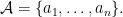 A singular proposition with respect to the basis
  will not remain singular if is extended by a number of new and independent features. Even if one keeps to the original set of pairwise options
  to pick out a new basis, the sets of linear propositions and positive propositions are both determined by the choice of basic propositions, and that entire determination is tantamount to the purely conventional choice of a cell as origin.
Resources
cc: Academia.edu • Cybernetics • Structural Modeling • Systems Science
cc: Conceptual Graphs • Laws of Form • Mathstodon • Research Gate

![[\mathcal{A}]](https://s0.wp.com/latex.php?latex=%5B%5Cmathcal%7BA%7D%5D&bg=ffffff&fg=000000&s=0&c=20201002)

![[\mathcal{A}].](https://s0.wp.com/latex.php?latex=%5B%5Cmathcal%7BA%7D%5D.&bg=ffffff&fg=000000&s=0&c=20201002)


 supplies the groundwork for any number of further extensions, beginning with the first order differential extension
  The construction of
  can be described in the following stages.
 is extended by a first order differential alphabet
  resulting in a first order extended alphabet
  defined as follows.
 is extended by a first order differential basis
  resulting in a first order extended basis
  defined as follows.
 is extended by a first order differential space or tangent space
  at each point of
  resulting in a first order extended space or tangent bundle space
  defined as follows.
![A^\bullet = [ a_1, \ldots, a_n ]](https://s0.wp.com/latex.php?latex=A%5E%5Cbullet+%3D+%5B+a_1%2C+%5Cldots%2C+a_n+%5D&bg=ffffff&fg=000000&s=0&c=20201002) is extended by a first order differential universe or tangent universe
is extended by a first order differential universe or tangent universe ![\mathrm{d}A^\bullet = [ \mathrm{d}a_1, \ldots, \mathrm{d}a_n ]](https://s0.wp.com/latex.php?latex=%5Cmathrm%7Bd%7DA%5E%5Cbullet+%3D+%5B+%5Cmathrm%7Bd%7Da_1%2C+%5Cldots%2C+%5Cmathrm%7Bd%7Da_n+%5D&bg=ffffff&fg=000000&s=0&c=20201002) at each point of
at each point of  resulting in a first order extended universe or tangent bundle universe
 ![\mathrm{E}A^\bullet ~=~ [ \mathrm{E}\mathcal{A} ] ~=~ [ \mathcal{A} ~\cup~ \mathrm{d}\mathcal{A} ] ~=~ [ a_1, \ldots, a_n, \mathrm{d}a_1, \ldots, \mathrm{d}a_n ].](https://s0.wp.com/latex.php?latex=%5Cmathrm%7BE%7DA%5E%5Cbullet+%7E%3D%7E+%5B+%5Cmathrm%7BE%7D%5Cmathcal%7BA%7D+%5D+%7E%3D%7E+%5B+%5Cmathcal%7BA%7D+%7E%5Ccup%7E+%5Cmathrm%7Bd%7D%5Cmathcal%7BA%7D+%5D+%7E%3D%7E+%5B+a_1%2C+%5Cldots%2C+a_n%2C+%5Cmathrm%7Bd%7Da_1%2C+%5Cldots%2C+%5Cmathrm%7Bd%7Da_n+%5D.&bg=ffffff&fg=000000&s=0&c=20201002)
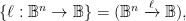
![[ \mathbb{B}^n \times \mathbb{D}^n ] ~=~ (\mathbb{B}^n \times \mathbb{D}^n\ +\!\!\to \mathbb{B}) ~=~ (\mathbb{B}^n \times \mathbb{D}^n, \mathbb{B}^n \times \mathbb{D}^n \to \mathbb{B}).](https://s0.wp.com/latex.php?latex=%5B+%5Cmathbb%7BB%7D%5En+%5Ctimes+%5Cmathbb%7BD%7D%5En+%5D+%7E%3D%7E+%28%5Cmathbb%7BB%7D%5En+%5Ctimes+%5Cmathbb%7BD%7D%5En%5C+%2B%5C%21%5C%21%5Cto+%5Cmathbb%7BB%7D%29+%7E%3D%7E+%28%5Cmathbb%7BB%7D%5En+%5Ctimes+%5Cmathbb%7BD%7D%5En%2C+%5Cmathbb%7BB%7D%5En+%5Ctimes+%5Cmathbb%7BD%7D%5En+%5Cto+%5Cmathbb%7BB%7D%29.&bg=ffffff&fg=000000&s=0&c=20201002)
 we arrive at the foothills of differential logic.
 to a set of two values, in other words, indicator functions of the form
  singular propositions are those singling out the minimal distinct regions of the universe, represented by single cells of the corresponding venn diagram.
 may be written as products:
 there are
  singular propositions. Their venn diagrams are shown in Figure 10.
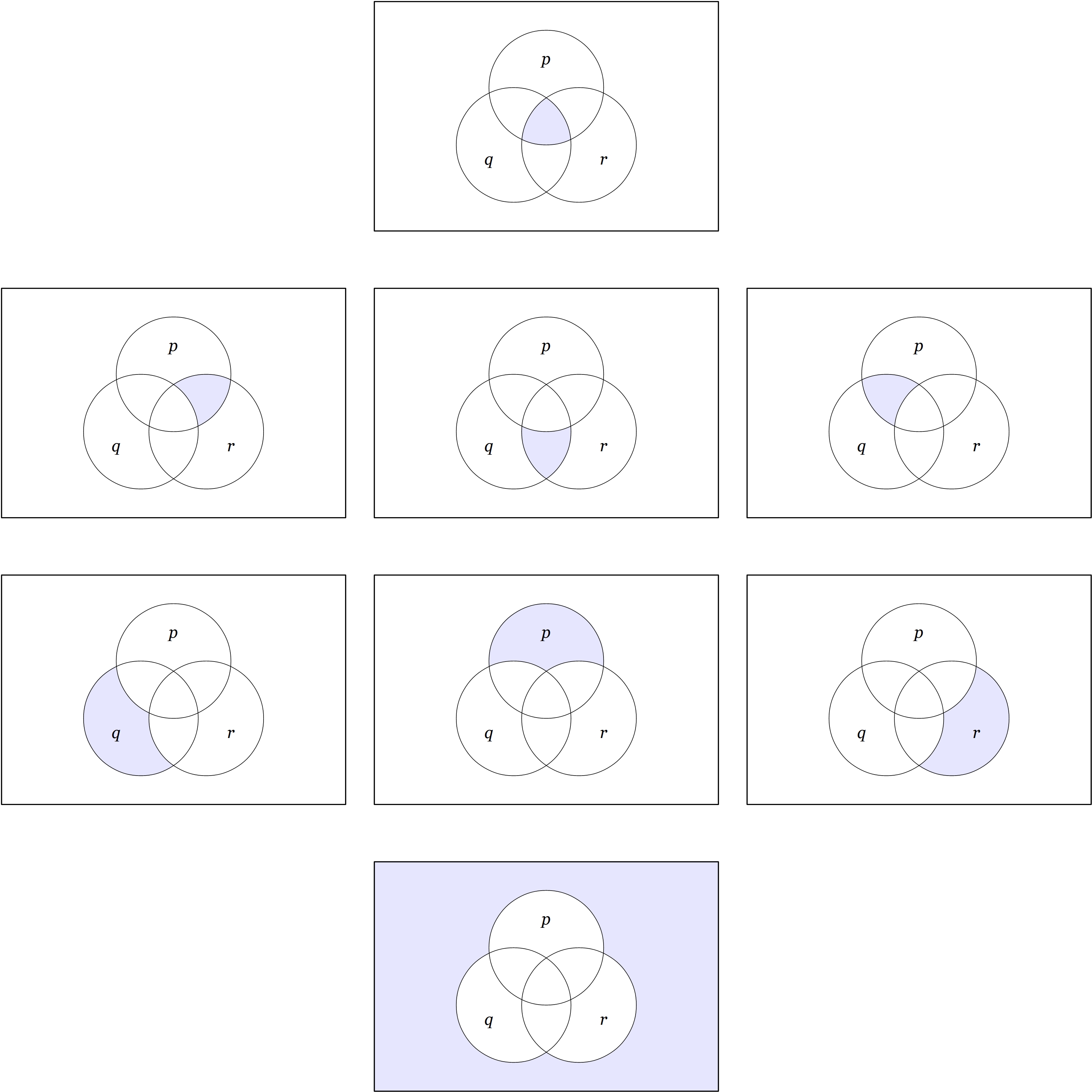

 and identical with the positive proposition of rank 3.


 may be written as products:


 respectively.
 function, which may be expressed by the form
  or by a simple
 may be written as sums:
 are added “modulo 2”, that is, in such a way that


 or by a simple
![A^\bullet = [a_1, \ldots, a_n]](https://s0.wp.com/latex.php?latex=A%5E%5Cbullet+%3D+%5Ba_1%2C+%5Cldots%2C+a_n%5D&bg=ffffff&fg=000000&s=0&c=20201002) qualified by the logical features
qualified by the logical features  There are
  accordingly pictured as all the ways of painting the cells of a venn diagram or the nodes of a hypercube with a palette of two colors.
 The signs are interpreted as denoting logical features, for example, properties of objects in the universe of discourse or simple propositions about those objects. Corresponding to the alphabet
 ![A^\bullet = [ \mathcal{A} ] = [ a_1, \ldots, a_n ].](https://s0.wp.com/latex.php?latex=A%5E%5Cbullet+%3D+%5B+%5Cmathcal%7BA%7D+%5D+%3D+%5B+a_1%2C+%5Cldots%2C+a_n+%5D.&bg=ffffff&fg=000000&s=0&c=20201002) It is useful to consider a universe of discourse as a categorical object incorporating both the set of points
It is useful to consider a universe of discourse as a categorical object incorporating both the set of points  implicit with the ordinary picture of a venn diagram on
  bearing the type
  which type designation may be abbreviated as
  or even more succinctly as
 ![[ \mathbb{B}^n ].](https://s0.wp.com/latex.php?latex=%5B+%5Cmathbb%7BB%7D%5En+%5D.&bg=ffffff&fg=000000&s=0&c=20201002) For convenience, the data type of a finite set on
For convenience, the data type of a finite set on ![[n]](https://s0.wp.com/latex.php?latex=%5Bn%5D&bg=ffffff&fg=000000&s=0&c=20201002) or
or 


