
The clock indicates the moment . . . . but what does
eternity indicate?
— Walt Whitman • Leaves of Grass
A One‑Dimensional Universe (concl.)
It might be thought an independent time variable needs to be brought in at this point but it is an insight of fundamental importance to realize the idea of process is logically prior to the notion of time. A time variable is a reference to a clock — a canonical, conventional process accepted or established as a standard of measurement but in essence no different than any other process. That raises questions of how different subsystems in a more global process can be brought into comparison and what it means for one process to serve the function of a local standard for others. Inquiries of that order serve but to wrap up our present puzzles in further riddles and are far too involved to be handled at our current level of approximation. We’ll return to them another time.
Observe how the secular inference rules, used by themselves, involve a loss of information, since nothing in them tells whether the momenta 


Resources
cc: Academia.edu • Cybernetics • Structural Modeling • Systems Science
cc: Conceptual Graphs • Laws of Form • Mathstodon • Research Gate
 is
is  If the feature
  is interpreted as applying to some object or state then the feature
  may be taken as an attribute of the same object or state which tells it is changing significantly with respect to the property
  as if it bore an “escape velocity” with respect to the state
  In practice, differential features acquire their meaning through a class of differential inference rules.
 will be true in the next moment of observation. Taken all together we have the fourfold scheme of inference shown below.
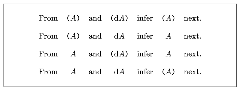
 be a logical basis containing one boolean variable or logical feature
  Corresponding to the basis
  which serves whenever we need to make explicit mention of the symbols used in our formulas and representations.
 of points (cells, vectors, interpretations) has cardinality
  and is isomorphic to
  Moreover,
  may be identified with the set of singular propositions
 is algebraically dual to
  Here,
Here,  is interpreted as denoting the constant function
  amounting to the linear proposition of rank
  while
while 
 of rank
  and
and  is understood as denoting the constant function
 propositions in the universe of discourse
 ![\mathcal{X}^\bullet = [\mathcal{X}],](https://s0.wp.com/latex.php?latex=%5Cmathcal%7BX%7D%5E%5Cbullet+%3D+%5B%5Cmathcal%7BX%7D%5D%2C&bg=ffffff&fg=000000&s=0&c=20201002) collectively forming the set
collectively forming the set 
![[\mathrm{E}\mathcal{A}]](https://s0.wp.com/latex.php?latex=%5B%5Cmathrm%7BE%7D%5Cmathcal%7BA%7D%5D&bg=ffffff&fg=000000&s=0&c=20201002) makes the task of solving differential propositions relatively straightforward. The solution set of the differential proposition
makes the task of solving differential propositions relatively straightforward. The solution set of the differential proposition  is the set of models
  in
in  Finding all models of
  the extended interpretations in
  which satisfy
  of a universe of discourse
 ![[\mathcal{A}]](https://s0.wp.com/latex.php?latex=%5B%5Cmathcal%7BA%7D%5D&bg=ffffff&fg=000000&s=0&c=20201002) is formed by taking the initial basis
is formed by taking the initial basis  together with the differential basis
  Thus we have the following formula.


![\mathrm{E}A^\bullet = [\mathrm{E}\mathcal{A}]](https://s0.wp.com/latex.php?latex=%5Cmathrm%7BE%7DA%5E%5Cbullet+%3D+%5B%5Cmathrm%7BE%7D%5Cmathcal%7BA%7D%5D&bg=ffffff&fg=000000&s=0&c=20201002) is the full collection of points and functions, or interpretations and propositions, based on the extended set of features
is the full collection of points and functions, or interpretations and propositions, based on the extended set of features  a fact summed up in the following notation.
![\mathrm{E}A^\bullet ~=~ [\mathrm{E}\mathcal{A}] ~=~ [a_1, \ldots, a_n, \mathrm{d}a_1, \ldots, \mathrm{d}a_n]](https://s0.wp.com/latex.php?latex=%5Cmathrm%7BE%7DA%5E%5Cbullet+%7E%3D%7E+%5B%5Cmathrm%7BE%7D%5Cmathcal%7BA%7D%5D+%7E%3D%7E+%5Ba_1%2C+%5Cldots%2C+a_n%2C+%5Cmathrm%7Bd%7Da_1%2C+%5Cldots%2C+%5Cmathrm%7Bd%7Da_n%5D&bg=ffffff&fg=000000&s=0&c=20201002)
 the following type.
 we arrive at the launchpad of our space explorations.

 taken by itself. In like fashion, the adjective extended or the substantive bundle is systematically attached to any construct associated with the full complement of
  features.
 sometimes written
  takes the form

 Strictly speaking, the name cotangent space is probably more correct for this construction but since we take up spaces and their duals in pairs to form our universes of discourse it allows our language to be pliable here.
 is a set consisting of two differential propositions,
  where
where  is a proposition with the logical value of
  Each component
  operating under the ordered correspondence
  A measure of clarity is achieved, however, by acknowledging the differential usage with a superficially distinct type
  whose sense may be indicated as follows.
 and
and  may appear to be identical sets of binary vectors, but taking a view at that level of abstraction would be like ignoring the qualitative units and the diverse dimensions that distinguish position and momentum, or the different roles of quantity and impulse.
 with a set of symbols for differential features, in effect basic changes capable of occurring in
 ![[\mathcal{A}].](https://s0.wp.com/latex.php?latex=%5B%5Cmathcal%7BA%7D%5D.&bg=ffffff&fg=000000&s=0&c=20201002) The additional symbols are taken to denote primitive features of change, qualitative attributes of motion, or proposals about the ways items in the universe of discourse may change or move in relation to features noted in the original alphabet.
The additional symbols are taken to denote primitive features of change, qualitative attributes of motion, or proposals about the ways items in the universe of discourse may change or move in relation to features noted in the original alphabet.
 in principle just an arbitrary set of symbols, disjoint from the initial alphabet
  and given the meanings just indicated.
