
Transformations of Discourse
It is understandable that an engineer should be completely absorbed in his speciality, instead of pouring himself out into the freedom and vastness of the world of thought, even though his machines are being sent off to the ends of the earth; for he no more needs to be capable of applying to his own personal soul what is daring and new in the soul of his subject than a machine is in fact capable of applying to itself the differential calculus on which it is based. The same thing cannot, however, be said about mathematics; for here we have the new method of thought, pure intellect, the very well‑spring of the times, the fons et origo of an unfathomable transformation.
— Robert Musil • The Man Without Qualities
Here we take up the general study of logical transformations, or maps relating one universe of discourse to another. In many ways, and especially as applied to the subject of intelligent dynamic systems, the argument will develop the antithesis of the statement just quoted. Along the way, if incidental to my ends, I hope the present essay can pose a fittingly irenic epitaph to the frankly ironic epigraph inscribed at its head.
The goal is to answer a single question: What is a propositional tangent functor? In other words, the aim is to develop a clear conception of what manner of thing would pass in the logical realm for a genuine analogue of the tangent functor, an object conceived to generalize as far as possible in the abstract terms of category theory the ordinary notions of functional differentiation and the all too familiar operations of taking derivatives.
As a first step we examine the types of transformations we already know as extensions and projections and we use their special cases to illustrate several styles of logical and visual representation which figure in the sequel.
Resources
cc: Academia.edu • Cybernetics • Structural Modeling • Systems Science
cc: Conceptual Graphs • Laws of Form • Mathstodon • Research Gate
 ‑gear curves, the indexing scheme results in the data of the next two Tables, showing one period for each orbit.
 where
where  may be read as a temporal parameter indicating the present time of the state and where
  is the decimal equivalent of the binary numeral
 with a subscript
  equal to the numerator of its rational index, taking for granted the constant denominator
  In that way the temporal succession of states can be reckoned by a parallel round‑up rule. Namely, if
  is any pair of adjacent digits in the state index
  then the value of
  in the next state is
 with the dyadic rationals (or the binary fractions) in the half-open interval
  Formally and canonically, a state
  is indexed by a fraction
  whose denominator is the power of two
  and whose numerator is a binary numeral formed from the coefficients of state in a manner to be described next.
 are the values
  for
for  where
where  is defined as identical to
  To form the binary index
  of the state
  Expressed in algebraic terms, the rational index
 Those are the trajectories generated subject to the dynamic law
  where it’s understood all higher order differences are equal to
 and all higher differences
  are fixed, the state vectors vary only with respect to their projections as points of
  Thus there is just enough space in a planar venn diagram to plot the orbits and show how they partition the points of
  It turns out there are just two possible orbits, of eight points each, as shown in the following Figure.

 The discussion to follow considers a class of trajectories having the property that
  for all
  greater than a fixed value
  and indulges in the use of a picturesque vocabulary to describe salient classes of those curves.
 exhibited at each point of any trajectory one may consider. With respect to any point of the corresponding curve let us call that highest order differential feature
  ‑gear curves.
 and
and 
 has a canonical expression
  in the set
  The tacit extension
  may then be expressed as a logical conjunction
  where
where  is a logical tautology using all the variables in
  The following Table shows how the tacit extensions
  of the propositions
  may be expressed in terms of the extended basis
![\text{Tacit Extension of}~ [A] ~\text{to}~ [A, \mathrm{d}A]](https://s0.wp.com/latex.php?latex=%5Ctext%7BTacit+Extension+of%7D%7E+%5BA%5D+%7E%5Ctext%7Bto%7D%7E+%5BA%2C+%5Cmathrm%7Bd%7DA%5D&bg=ffffff&fg=000000&s=1&c=20201002)
![Tacit Extension of [A] to [A, dA]](https://inquiryintoinquiry.com/wp-content/uploads/2023/12/differential-logic-e280a2-tacit-extensions.png)
 the above analysis has an interesting interpretation. The tacit extension takes us from thinking about a particular state, like
  or
or  to considering the collection of outcomes, the outgoing changes or singular dispositions springing or stemming from that state.
 even though they share the same logical expression. Naturally, we want to maintain the logical equivalence of expressions representing the same proposition while appreciating the full diversity of a proposition’s functional and typical representatives. Both perspectives, and all the levels of abstraction extending through them, have their reasons, as will develop in time.
 is a subset of another basis
  we say any proposition
  has a tacit extension to a proposition
  and we say the space
  has an automatic embedding within the space
 is defined in such a way that
  puts the same constraint on the variables of
  as the proposition
  initially put on
  while it puts no constraint on the variables of
  and
and  the tacit extension from
 where the bases
  may be silent.
![[\mathrm{E}\mathcal{X}] = [A, \mathrm{d}A].](https://s0.wp.com/latex.php?latex=%5B%5Cmathrm%7BE%7D%5Cmathcal%7BX%7D%5D+%3D+%5BA%2C+%5Cmathrm%7Bd%7DA%5D.&bg=ffffff&fg=000000&s=0&c=20201002)
 of cardinality
  generates the terms of description for the extended space
  of cardinality
  according to the following series of equations.
![\begin{array}{lll} \mathrm{E}X & = & \langle A, \mathrm{d}A \rangle \\[4pt] & = & \{ \texttt{(} A \texttt{)}, A \} ~\times~ \{ \texttt{(} \mathrm{d}A \texttt{)}, \mathrm{d}A \} \\[4pt] & = & \{ \texttt{(} A \texttt{)(} \mathrm{d}A \texttt{)},~ \texttt{(} A \texttt{)} \mathrm{d}A,~ A \texttt{(} \mathrm{d}A \texttt{)},~ A ~ \mathrm{d}A \}. \end{array}](https://s0.wp.com/latex.php?latex=%5Cbegin%7Barray%7D%7Blll%7D++%5Cmathrm%7BE%7DX+%26+%3D+%26+%5Clangle+A%2C+%5Cmathrm%7Bd%7DA+%5Crangle++%5C%5C%5B4pt%5D++%26+%3D+%26+%5C%7B+%5Ctexttt%7B%28%7D+A+%5Ctexttt%7B%29%7D%2C+A+%5C%7D+%7E%5Ctimes%7E+%5C%7B+%5Ctexttt%7B%28%7D+%5Cmathrm%7Bd%7DA+%5Ctexttt%7B%29%7D%2C+%5Cmathrm%7Bd%7DA+%5C%7D++%5C%5C%5B4pt%5D++%26+%3D+%26+%5C%7B+%5Ctexttt%7B%28%7D+A+%5Ctexttt%7B%29%28%7D+%5Cmathrm%7Bd%7DA+%5Ctexttt%7B%29%7D%2C%7E++%5Ctexttt%7B%28%7D+A+%5Ctexttt%7B%29%7D+%5Cmathrm%7Bd%7DA%2C%7E++A+%5Ctexttt%7B%28%7D+%5Cmathrm%7Bd%7DA+%5Ctexttt%7B%29%7D%2C%7E++A+%7E+%5Cmathrm%7Bd%7DA+%5C%7D.++%5Cend%7Barray%7D&bg=ffffff&fg=000000&s=0&c=20201002)
 at root isomorphic to
  An element of
 ![\mathrm{E}X^\bullet = [A, \mathrm{d}A]](https://s0.wp.com/latex.php?latex=%5Cmathrm%7BE%7DX%5E%5Cbullet+%3D+%5BA%2C+%5Cmathrm%7Bd%7DA%5D&bg=ffffff&fg=000000&s=0&c=20201002) the basic dispositions in
the basic dispositions in  each of type
  There are
  propositions in
  as detailed in the following Table.
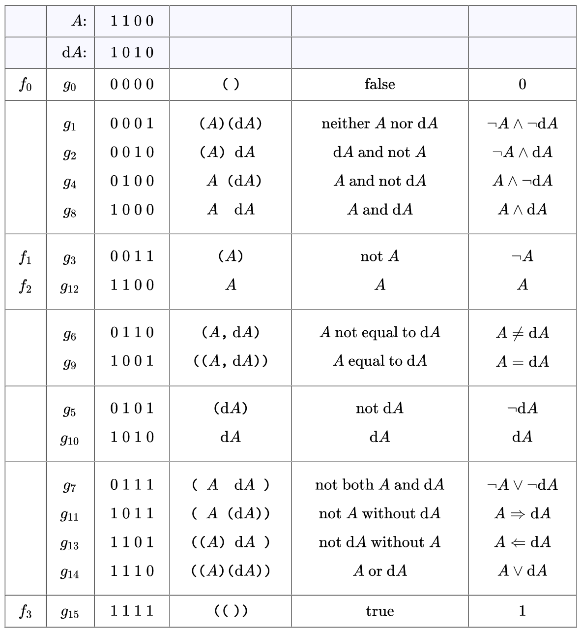
 Thus the first set of propositions
  is automatically embedded in the present set
  and the corresponding inclusions are indicated at the far left margin of the Table.