Casual Introduction (cont.)

Figure 3 extends the basis of description for the space to a set of two qualities and the corresponding terms of description to an alphabet of two symbols

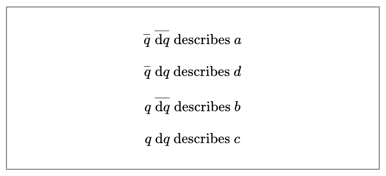
Any propositional calculus over two basic propositions allows for the expression of sixteen propositions all together.  Salient among those propositions in the present setting are the four which single out the individual sample points at the initial moment of observation.  Table 4 lists the initial state descriptions, using overlines to express logical negations.

cc: FB | Differential Logic • Laws of Form • Mathstodon • Academia.edu
cc: Conceptual Graphs • Cybernetics • Structural Modeling • Systems Science