Differential Logic

Differential Fields

The structure of a differential field may be described as follows. With each point of $X$ there is associated an object of the following type: a proposition about changes in $X,$ that is, a proposition $g : \mathrm{d}X \to \mathbb{B}.$ In that frame of reference, if ${X^\bullet}$ is the universe generated by the set of coordinate propositions $\{ p, q \}$ then $\mathrm{d}X^\bullet$ is the differential universe generated by the set of differential propositions $\{ \mathrm{d}p, \mathrm{d}q \}.$ The differential propositions $\mathrm{d}p$ and $\mathrm{d}q$ may thus be interpreted as indicating $``\text{change in}~ p"$ and $``\text{change in}~ q",$ respectively.

A differential operator $\mathrm{W},$ of the first order type we are currently considering, takes a proposition $f : X \to \mathbb{B}$ and gives back a differential proposition $\mathrm{W}f : \mathrm{E}X \to \mathbb{B}.$ In the field view of the scene, we see the proposition $f : X \to \mathbb{B}$ as a scalar field and we see the differential proposition $\mathrm{W}f : \mathrm{E}X \to \mathbb{B}$ as a vector field, specifically, a field of propositions about contemplated changes in $X.$

The field of changes produced by $\mathrm{E}$ on $pq$ is shown in the following venn diagram.

$\text{Enlargement}~ \mathrm{E}(pq) : \mathrm{E}X \to \mathbb{B}$

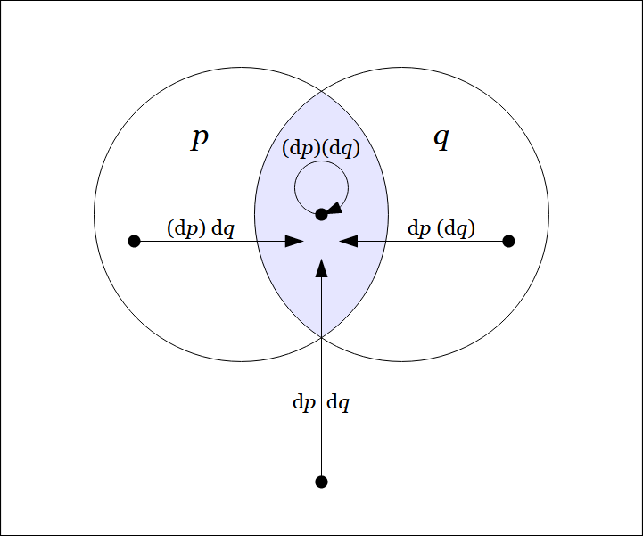
$\begin{array}{rcccccc} \mathrm{E}(pq) & = & p & \cdot & q & \cdot & \texttt{(} \mathrm{d}p \texttt{)(} \mathrm{d}q \texttt{)} \\[4pt] & + & p & \cdot & \texttt{(} q \texttt{)} & \cdot & \texttt{(} \mathrm{d}p \texttt{)~} \mathrm{d}q \texttt{~} \\[4pt] & + & \texttt{(} p \texttt{)} & \cdot & q & \cdot & \texttt{~} \mathrm{d}p \texttt{~(} \mathrm{d}q \texttt{)} \\[4pt] & + & \texttt{(} p \texttt{)} & \cdot & \texttt{(} q \texttt{)} & \cdot & \texttt{~} \mathrm{d}p \texttt{~~} \mathrm{d}q \texttt{~} \end{array}$

The differential field $\mathrm{E}(pq)$ specifies the changes which need to be made from each point of $X$ in order to reach one of the models of the proposition $pq,$ that is, in order to satisfy the proposition $pq.$

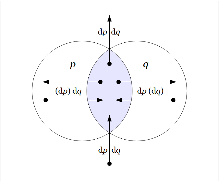
The field of changes produced by $\mathrm{D}$ on $pq$ is shown in the following venn diagram.

$\text{Difference}~ \mathrm{D}(pq) : \mathrm{E}X \to \mathbb{B}$

$\begin{array}{rcccccc} \mathrm{D}(pq) & = & p & \cdot & q & \cdot & \texttt{((} \mathrm{d}p \texttt{)(} \mathrm{d}q \texttt{))} \\[4pt] & + & p & \cdot & \texttt{(} q \texttt{)} & \cdot & \texttt{~(} \mathrm{d}p \texttt{)~} \mathrm{d}q \texttt{~~} \\[4pt] & + & \texttt{(} p \texttt{)} & \cdot & q & \cdot & \texttt{~~} \mathrm{d}p \texttt{~(} \mathrm{d}q \texttt{)~} \\[4pt] & + & \texttt{(} p \texttt{)} & \cdot & \texttt{(}q \texttt{)} & \cdot & \texttt{~~} \mathrm{d}p \texttt{~~} \mathrm{d}q \texttt{~~} \end{array}$

The differential field $\mathrm{D}(pq)$ specifies the changes which need to be made from each point of $X$ in order to feel a change in the felt value of the field $pq.$

Resources

cc: Academia.edu • Cybernetics • Structural Modeling • Systems Science
cc: Conceptual Graphs • Laws of Form • Ma^thstodon • Research Gate

	Survey of Semiotics,… on Sign Relations • Semiotic Equi…
	Survey of Semiotics,… on Sign Relations • Semiotic Equi…
	Sign Relations • Sem… on Survey of Semiotics, Semiosis,…
	Survey of Semiotics,… on Sign Relations • Semiotic Equi…
	Sign Relations • Sem… on Survey of Semiotics, Semiosis,…
	Sign Relations • Sem… on Survey of Semiotics, Semiosis,…
	Survey of Semiotics,… on Sign Relations • Semiotic Equi…
	Sign Relations • Sem… on Survey of Semiotics, Semiosis,…
	Survey of Semiotics,… on Systems of Interpretation •…
	Survey of Semiotics,… on Sign Relations, Triadic Relati…

M	T	W	T	F	S	S
				1	2	3
4	5	6	7	8	9	10
11	12	13	14	15	16	17
18	19	20	21	22	23	24
25	26	27	28	29	30