
Differential Expansions of Propositions
Panoptic View • Enlargement Maps
The enlargement or shift operator 

A suitably generic definition of the extended universe of discourse is afforded by the following set‑up.
![\begin{array}{cccl} \text{Let} & X & = & X_1 \times \ldots \times X_k. \\[6pt] \text{Let} & \mathrm{d}X & = & \mathrm{d}X_1 \times \ldots \times \mathrm{d}X_k. \\[6pt] \text{Then} & \mathrm{E}X & = & X \times \mathrm{d}X \\[6pt] & & = & X_1 \times \ldots \times X_k ~\times~ \mathrm{d}X_1 \times \ldots \times \mathrm{d}X_k \end{array}](https://s0.wp.com/latex.php?latex=%5Cbegin%7Barray%7D%7Bcccl%7D++%5Ctext%7BLet%7D+%26+X+%26+%3D+%26+X_1+%5Ctimes+%5Cldots+%5Ctimes+X_k.++%5C%5C%5B6pt%5D++%5Ctext%7BLet%7D+%26+%5Cmathrm%7Bd%7DX+%26+%3D+%26+%5Cmathrm%7Bd%7DX_1+%5Ctimes+%5Cldots+%5Ctimes+%5Cmathrm%7Bd%7DX_k.++%5C%5C%5B6pt%5D++%5Ctext%7BThen%7D+%26+%5Cmathrm%7BE%7DX+%26+%3D+%26+X+%5Ctimes+%5Cmathrm%7Bd%7DX++%5C%5C%5B6pt%5D++%26+%26+%3D+%26+X_1+%5Ctimes+%5Cldots+%5Ctimes+X_k+%7E%5Ctimes%7E+%5Cmathrm%7Bd%7DX_1+%5Ctimes+%5Cldots+%5Ctimes+%5Cmathrm%7Bd%7DX_k++%5Cend%7Barray%7D&bg=ffffff&fg=000000&s=0&c=20201002)
For a proposition of the form 


The differential variables 


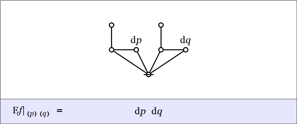
In the example of logical conjunction, 


Given that the above expression uses nothing more than the boolean ring operations of addition and multiplication, it is permissible to “multiply things out” in the usual manner to arrive at the following result.

To understand what the enlarged or shifted proposition means in logical terms, it serves to go back and analyze the above expression for 


Collating the data of that analysis yields a boolean expansion or disjunctive normal form (DNF) equivalent to the enlarged proposition


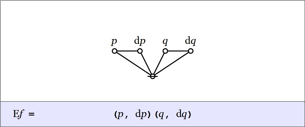
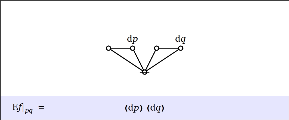
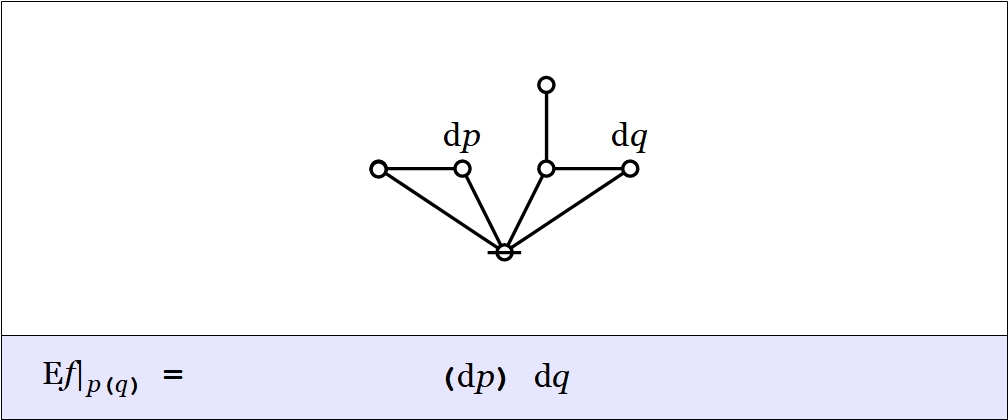
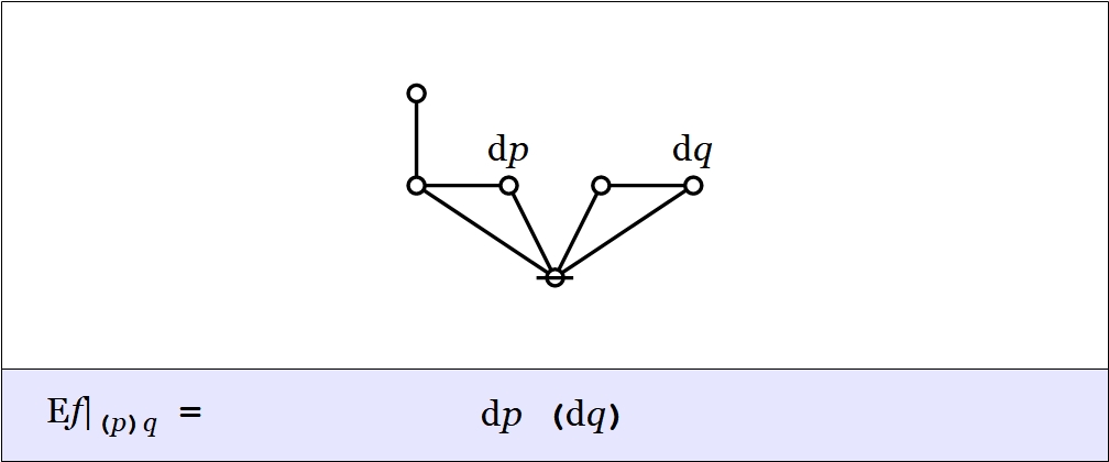
Here is a summary of the result, illustrated by means of a digraph picture, where the “no change” element 

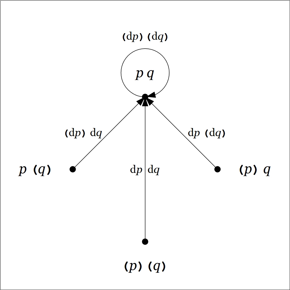
![\begin{array}{rcccccc} f & = & p & \cdot & q \\[4pt] \mathrm{E}f & = & p & \cdot & q & \cdot & \texttt{(} \mathrm{d}p \texttt{)(} \mathrm{d}q \texttt{)} \\[4pt] & + & p & \cdot & \texttt{(} q \texttt{)} & \cdot & \texttt{(} \mathrm{d}p \texttt{)} \texttt{~} \mathrm{d}q \texttt{~} \\[4pt] & + & \texttt{(} p \texttt{)} & \cdot & q & \cdot & \texttt{~} \mathrm{d}p \texttt{~} \texttt{(} \mathrm{d}q \texttt{)} \\[4pt] & + & \texttt{(} p \texttt{)} & \cdot & \texttt{(} q \texttt{)} & \cdot & \mathrm{d}p \texttt{~~} \mathrm{d}q \end{array}](https://s0.wp.com/latex.php?latex=%5Cbegin%7Barray%7D%7Brcccccc%7D++f+%26+%3D+%26+p++%26+%5Ccdot+%26+q++%5C%5C%5B4pt%5D++%5Cmathrm%7BE%7Df+%26+%3D+%26+p++%26+%5Ccdot+%26++q++%26+%5Ccdot+%26++%5Ctexttt%7B%28%7D+%5Cmathrm%7Bd%7Dp+%5Ctexttt%7B%29%28%7D+%5Cmathrm%7Bd%7Dq+%5Ctexttt%7B%29%7D++%5C%5C%5B4pt%5D++%26+%2B+%26++p++%26+%5Ccdot+%26+%5Ctexttt%7B%28%7D+q+%5Ctexttt%7B%29%7D++%26+%5Ccdot+%26++%5Ctexttt%7B%28%7D+%5Cmathrm%7Bd%7Dp+%5Ctexttt%7B%29%7D+%5Ctexttt%7B%7E%7D+%5Cmathrm%7Bd%7Dq+%5Ctexttt%7B%7E%7D++%5C%5C%5B4pt%5D++%26+%2B+%26++%5Ctexttt%7B%28%7D+p+%5Ctexttt%7B%29%7D+%26+%5Ccdot+%26++q++%26+%5Ccdot+%26++%5Ctexttt%7B%7E%7D+%5Cmathrm%7Bd%7Dp+%5Ctexttt%7B%7E%7D+%5Ctexttt%7B%28%7D+%5Cmathrm%7Bd%7Dq+%5Ctexttt%7B%29%7D++%5C%5C%5B4pt%5D++%26+%2B+%26++%5Ctexttt%7B%28%7D+p+%5Ctexttt%7B%29%7D+%26+%5Ccdot+%26+%5Ctexttt%7B%28%7D+q+%5Ctexttt%7B%29%7D++%26+%5Ccdot+%26+%5Cmathrm%7Bd%7Dp+%5Ctexttt%7B%7E%7E%7D+%5Cmathrm%7Bd%7Dq++%5Cend%7Barray%7D&bg=ffffff&fg=000000&s=0&c=20201002)
We may understand the enlarged proposition

Resources
cc: Academia.edu • Cybernetics • Structural Modeling • Systems Science
cc: Conceptual Graphs • Laws of Form • Mathstodon • Research Gate

Pingback: Survey of Differential Logic • 7 | Inquiry Into Inquiry
Pingback: Survey of Differential Logic • 7 | Inquiry Into Inquiry
Pingback: Survey of Differential Logic • 8 | Inquiry Into Inquiry
Pingback: Survey of Differential Logic • 8 | Systems Community of Inquiry